Chapter 15

Auditory image fundamentals

15.1 Introduction

In the previous chapters, we established a theoretical and quantitative analytical basis for temporal imaging in the auditory system, along with a firm basis for an auditory-relevant notion of coherence. The original temporal imaging theory applies directly to individual samples or pulses, but we qualitatively extended it to include nonuniform sampling, in order to make better use of the modulation transfer functions that can be applied over longer durations than single samples. It highlighted the distinction between coherent and incoherent sound, which can be traced to the inherent defocus of the auditory system (and its preferential phase locking), and is supported by empirical data about the temporal modulation transfer functions. This distinction indicates that there is an increased sensitivity to high frequencies that modulate coherent carriers in comparison to incoherent carriers.

There appears to be a built-in system that may be more optimal for coherent than for incoherent sound detection, insofar as the within-channel imaging is analyzed. This is so because of the relative broader bandwidth of the coherent modulation transfer function (MTF), which is completely flat in the effective passband—at modulation frequencies that do not get resolved in adjacent filters. In contrast, incoherent carriers carry random modulation noise at low frequencies and tend to have poorer sensitivity, unless information from several channels is pooled together. These observations are not trivially integrated when it comes to the design of the complete auditory imaging system. Analogy to spatial imaging in vision is also not helpful, as vision is strictly incoherent. In fact, incoherent-illumination imaging normally produces superior images to coherent illumination, which produces images that are much more sensitive to diffraction effects and speckle noise (e.g., dust particles on the objects or on the system elements that become visible in coherent illumination). Additionally, incoherent imaging is strictly intensity-based (i.e., linear in intensity), whereas coherent imaging is amplitude-based (linear in amplitude), although its final product is usually an intensity image as well. Direct comparison between visual and auditory imaging can only be made based on intensity images, but because of the longstanding confusion about the role of phase in hearing (§6.4.2), it is not immediately clear that amplitude imaging does not have a role in hearing and that the comparison is valid.

Many natural sound sources are coherent, but the acoustic environment and medium tend to decohere their radiated sound through reflections, dispersion, and absorption (§3.4). Other sounds of interest are generated incoherently at the source, but their received coherence depends on the bandwidth of the sound and the filters that analyze it. Therefore, we would like to formulate the action of auditory imaging, so that it can differentially respond to arbitrary levels of signal coherence. The effects of complete coherence or incoherence are well known (mainly for stationary signals), but much of the intuition in them may be lost because they are usually not framed as part of an auditory-relevant coherence theory. This means that for the majority of signals that are neither coherent nor incoherent there are no presently available heuristics that can be used to analyze them. We would like to provide some conceptual tools that bridge this gap in intuitive understanding of realistic acoustic object imaging.

This chapter follows a broad arc that encompasses several key topics in auditory imaging. It begins with discussions about sharp and blurry auditory images, which enables us to make sense out of the substantial defocus that is built into the auditory system. Suprathreshold imaging is then discussed, based on an extrapolation of threshold-level masking responses. The notion of polychromatic images is applied to hearing by way of analogy with a number of known phenomena that are reframed appropriately to support it. The special case of acoustic objects that elicit pitch is briefly reviewed and is also reframed with imaging in mind. Then, several sections deal with various polychromatic and monochromatic aberrations, as well as an interpretation of the depth of focus of the system. Finally, we provide a few rules of thumb that aid the intuition of how images are produced in the system.

15.2 Sharpness and blur in the hearing literature

Sharpness and blur are central concepts when discussing the optics of the eye (e.g., Le Grand and El Hage, 1980; Packer and Williams, 2003, pp. 52–61) and imaging systems in general. If a visual system does not produce sufficiently sharp images due to blur, it can cause various levels of disability if not corrected. Therefore, identifying the auditory analogs of sharpness and blur—should they exist—may be a powerful stepping stone in understanding how the ear works and where things can go wrong.

Currently, there is no analogous concept in psychoacoustics for sharpness that resembles the optical one and references to it in the auditory literature are scarce. Sharpness was introduced in psychoacoustics as a consistently large factor of timbre (von Bismarck, 1974). Ranging on a subjective scale between dull and sharp, sharpness was modeled using the first moment of the sum of the loudness function in all critical bands, where the high frequency content above 16 Bark (3.4 kHz) affected the rated sharpness of the stimuli tested—typically, noise and complex tones (Fastl and Zwicker, 2007; pp. 239–243). These conceptualizations of psychoacoustic sharpness appear to be irrelevant to the present discussion.

The antonymous notion of sharpness, blur, is more frequently encountered in the hearing literature, and is closer to how it is used in imaging. It is perhaps because of the association of the convolution with blurring operations that makes this term somewhat more commonplace in hearing research (e.g., Stockham et al., 1975). For example, blur is occasionally invoked in the context of modulation transfer function fidelity that is impacted by room acoustics (Houtgast and Steeneken, 1985), or through manipulation of the speech envelope through modulation filtering (Drullman et al., 1994a; Drullman et al., 1994b). Similarly, in bird vocalizations, the in-situ degradation of envelope patterns over time and distance were quantified and referred to as blur (Dabelsteen et al., 1993). Another typical usage was exemplified by Simmons et al. (1996), who referred to the blurring effects of the long integration window on the perception of minute features in the echoes perceived by bats over durations shorter than 0.5 ms. Similar references to temporal or spectral blur occasionally appear in the hearing literature. For example, Carney (2018) raised the question of whether there is an auditory analog to the visual accommodation system that reacts and corrects blur to achieve (attentional) focus.

A single study tested the focus of sound sources directly. A subjective rating of the perceived source focus of anechoic speech superposed either with a specular or with a diffuse reflection was obtained in Visentin et al. (2020). Subjects were instructed that focus “should be considered as the distinction between a “clear” or “well-defined” sound source and a “blurred” sound image.” Two clear patterns were observed. First, when the angle of diffuse reflection was increased (from \(34^\circ\) to \(79^\circ\)), the rated focus dropped to the point that it became equal to the specular reflection. Likely, at large angles the reflection was coherent-like and interfered with the source definition. Similarly, the rated focus was also correlated with the interaural time difference (ITD) averaged over 500, 1000, and 2000 Hz octave bands. So the focus was rated highest for ITD when it was about 0. As was argued in §8.5, the ITD directly quantifies spatial coherence. So maximum coherence correlated with the maximum perceived focus, as long as the source direction is unambiguous. Incidentally, the focus highly correlated (\(r=0.84\)) with speech intelligibility, which was also highly correlated with rated loudness.

Clarity is an altogether different concept, which is probably associated with sharpness to some extent, and is more common in different audio-quality and audiometric evaluations. It was designated as a fundamental component of hearing-aid performance that is hampered by noise and distortion (Katz et al., 2015; p. 61)—two factors that affect the imaging quality independently (Blackledge, 1989; pp. 8–9). In room acoustics, clarity (\(C_{80}\)) is often used to estimate the power of the earliest portion of the room impulse response in which single reflections are still relatively prominent, in comparison with the late portion (after 80 ms) (Kuttruff, 2017; pp. 169–170). This quantity has been used to estimate the sound transparency in concert hall acoustics. Clarity is also used more informally in audio quality evaluations (Bech and Zacharov, 2006; Toole, 2009), and was defined by Bech and Zacharov (2006) as: “Clarity—This attribute describes if the sound sample appears clear or muffled, for example, if the sound source is perceived as covered by something.”. Muffled sounds often suggest high frequency content roll-off due to absorption—perhaps the opposite quality to Bismarck's sharpness. High modulation frequency roll-off is also a common feature of blur in spatial imaging, as the removal of high spatial frequencies causes the blur of sharp edges.

15.3 Sharpness, blur, and aberrations of auditory images

In vision, sharpness characterizes static images and can be extended to moving images without much difficulty. In hearing, even static images (with constant temporal envelopes, as pure tones) unfold over time, which is physically, perceptually, and conceptually unlike images of still visual objects, despite the mathematical parallels garnered by the space-time duality. Although we now have the imaging transform of a single pulse or sample, the short duration of the aperture does not truly allow for any appreciation of the image sharpness. Therefore, it is only through the concatenation of samples over time that auditory sharpness can be sensibly established. Still, it is much simpler to analyze the conditions for the loss of sharpness—the creation of blur—than those that give rise to sharpness. If the sources of auditory blur are negligible or altogether absent, relative sharpness can be argued for and established. In other words, we can define auditory sharpness by negation: The auditory image is sharp when different sources of image blur are either negligible or imperceptible. Therefore, the remainder of this chapter is dedicated to elucidating the different forms of blur and related aberrations that can be found in human hearing.

15.3.1 The two limits of optical blur

In both spatial and temporal imaging, the information about blur is fully contained in the impulse response function (or the point spread function of the two spatial dimensions), which relates a point in the object plane to a region in the image plane. In two dimensions, the effect of blur is to transform a point into a disc. As we saw in §13, the point spread function is fully determined by the pupil function of the imaging system and, specifically, it depends on the neural group-delay dispersion (analogous to the distance between the lens and the screen in spatial optics).

There are two limits that characterize the possible blur in the image. When the aperture is large compared to the light wavelength, the image is susceptible to geometrical blur. It can be explained by considering the different paths that exist between a point of the object to the image, which do not all meet in one mathematical point. Thus, in geometrical blur, multiple non-overlapping copies of the image are overlaid in the image plane. Consequently, the fine details and sharp edges of the object are smeared and the imaged point appears blurry. Geometric blur can be further specified according to the exact transformation that causes an object point to assume a distorted shape on the image plane. These distortions are called aberrations and among them, defocus is the simplest one that causes blur.

In the other extreme, when the aperture size is comparable or smaller than the wavelength, the image becomes susceptible to effects of diffraction. A point then turns into a disc with oscillating bands of light and shadow (fringes), which makes fine details less well-defined, and hence, blurry.

The aperture size for an ideal imaging system should be designed to produce blur between these two limits. An image that does not have any aberrations is referred to as diffraction-limited.

15.3.2 Contrast and blur

It is worthwhile to dwell on the two image fidelity characteristics that often appear together—contrast and blur—and elucidate their differences. Contrast quantifies the differences in intensity between the brightest and darkest points in the image, or a part thereof. Hence, it is a measure of the dynamic range of the image, which ideally maps the dynamic range of the object, so that intensity information is not lost in the imaging process. As the image is made of spatial modulations, contrast is quantified with visibility (Eq. §7.1), which we also referred to as modulation depth (§6.4.1).

Blur refers to the transformation that the image undergoes that makes it different from a simple scaling transformation of the object. The effects of geometrical and diffractive blurs are not the same here, though. In geometrical blur, the envelope broadens, as spectral components share energy with neighboring components and overall distort the image, while retaining its general shape. In diffractive blur, new spectral components can emerge in the envelope that are not part of the original object, but appear due to wave interaction with small features in the system or object that have similar dimensions to the wavelength of light carrier. In both cases, both the envelope and its spectrum change due to blur.

While blur and contrast can and often interact, they represent two different dimensions of the imaging system and we will occasionally emphasize one and not the other. Contrast does not interact directly with the spectral content of the image, whereas blur does. Note that when the envelope spectrum is imaged, it is scaled with magnification, which is a transformation that is integral to the imaging operation and does not entail blur or contrast effects.

15.3.3 Auditory blur and aberrations

The temporal auditory image blur can be understood in analogous terms to spatial blur by substituting the aperture size with aperture time and diffraction with dispersion. Thus, the temporal image can be geometrically blurred if the aperture time is much longer than the period of the sound. If it has no aberrations, then it can be considered to be dispersion-limited. A very short aperture with respect to the period may produce audible dispersion effects, at least when fine sound details are considered. Thus, a good temporal imaging design should strike a balance between geometrical blur and blur from dispersion. In fact, what we saw earlier is that the system is set far from this optimum, since it is significantly skewed toward a geometrical blur, which is seen in the significant defocus we obtained—an aberration (§12.3, §12.5, and §13.2.2).

However, things get more complicated with sound in ways that do not have analogs in vision. The most significant difference, as was repeatedly implied throughout the text, is that unlike visual imaging that is completely incoherent, sound is partially coherent, but some of the most important sounds to humans have strong coherent components in them. As was shown in §13.4 and will be discussed in §15.5, the defocus blurs incoherent objects more than it does coherent ones. Thus, it can be used to differentiate types of coherence by design, instead of achieving nominally uniform blur across arbitrary degrees of input coherence.

The second complication in sound is due to the nonuniform temporal sampling by the auditory nerve that replaces the fixed (yet still nonuniform) spatial sampling in the retina. The loss of high modulation frequency information from the image because of insufficient (slow) sampling rate (and possibly other factors) can be a source of blur as well, which is neither dispersive nor geometrical per se. This effect will not be considered here beyond the earlier discussion about its effects on the modulation transfer function in §14.8.

Another nonstandard form of geometrical blur may occur if the sampling rate and the aperture time are mismatched, so that consecutive samples overlap (i.e., the duty cycle is larger than 100%). Effectively, this kind of blur is produced outside of the auditory system in the environment through reverberation, where multiple reflections of the object are superimposed in an irregular manner that decoheres the signal (§3.4.4).

A combined form of geometrical and dispersive blur is caused by chromatic aberration—when the monochromatic images from the different channels are not exactly overlapping or synchronized, which gives rise to the blurring of onsets and other details. Virtually all polychromatic (broadband) optical systems have some degree of chromatic aberration and the possibility of encountering it in hearing will be explored in §15.10.

Image blur may be caused by other aberrations, as a result of the time lens imperfect quadratic curvature, when its phase function contains higher-order terms in its Taylor expansion (see Eq. §10.27). Similarly, phase distortion may be a problem in the group dispersive segments of the cochlea or the neural pathways, if their Taylor expansion around the carrier (Eq. §10.6) has higher terms (Bennett and Kolner, 2001). While this large family of aberrations is very well-studied in optics and vision, the existence of their temporal aberrations in hearing is difficult to identify at the present state of knowledge. They will be explored in §15.9.

In general, blurring effects can be also produced externally to the temporal imaging system. Outside of the system, it can accrue over large propagation distances, and likely occurs in turbulent atmospheric conditions (§3.4.2). Phase distortion can also be the result of individual reflections from surfaces (§3.4.3). As was reviewed in §11.2, the plane-wave approximation gradually breaks down in the ear canal above 4 kHz, which means that modulation information may be carried by different modes with different group velocities. This situation causes a so-called dispersion distortion in optics (§10.4), and may theoretically cause distortion and blur also in hearing at high frequencies.

15.4 Suprathreshold masking, contrast, and blur

Few auditory phenomena have received more attention in psychoacoustic research than masking. Beyond the curious nature of its effects, interest has stemmed from the usefulness of masking in indirectly estimating many hearing parameters and thereby inferring various aspects regarding the auditory system signal processing. Additionally, it has been implied that masking effects can be generalized to everyday hearing and can significantly impact its outcomes—especially with hearing impairments.

The definition of masking normally refers to an increase in the threshold of a stimulus in the presence of another sound (Oxenham, 2014). However, the change in threshold can be caused by more than one process and several peripheral and neural mechanisms have been considered in literature in different contexts (Oxenham, 2001; Moore, 2013). But since the discussion of masking is strictly framed around the change of threshold, it leaves out a no-less important discussion about how audible, or suprathreshold, signals sound in the presence of masking. Put differently, a complete knowledge of the masking threshold does not necessarily mean that the suprathreshold signal combined with the masker is going to sound identical to a lower-level version of the original signal in the absence of masking.

We can think of four general classes of interactions between masker and signal, or even more generally, between any two acoustic objects.

The first class of masking relates to masking that only causes the signal to sound less intense, while it is otherwise unchanged when it is presented above its masking threshold. This effect can be analogized to the apparent dimming of one object in the presence of another (e.g., viewing a remote star in broad daylight). In a perfectly linear system, amplification of the dim target leads to its perfect recovery with no distortion or loss of information. When the system exhibits (nonlinear) dynamic range compression, perfect recovery of the envelope requires variable amplification (i.e., expansion) and may be impossible to realize in practice. When the sound in question is modulated, this is akin to loss of contrast—the difference between the envelope maximum and minimum. Loss of contrast can also happen if only part of the modulated sound is masked, whereas the rest is above threshold. Or, it can take place if the loudest parts of the sound saturate and do not allow for a linear mapping of intensity. In any case, this type of masking is strictly incoherent, as the signal and masker only interact by virtue of intensity superposition.

In the second class of masking, the suprathreshold signal interacts with the masker and its fine details change as a result, even if they are still recognizable as the target sound. This can obviously happen only if the two sounds interfere, which is possible when they are mutually coherent or partially coherent within the aperture stop of the relevant channel(s). As this phenomenon involves interference, the corresponding optical analogy here is diffraction blur. Note that this analogy does not specify the conditions for an interference-like response, which is usually referred to as suppression phenomena in hearing. Suppression is thought to involve nonlinearities, which extend beyond the normal bandwidth of the auditory channel. In this case, the response may not be obviously interpreted as interference, since it can also be caused by inhibition in the central pathways, which may produce a similar perceptual effect, but have a different underlying mechanism. In his seminal paper of two-tone suppression masking, Houtgast (1972) compared it to Mach bands in vision, which appear as change in contrast around the object edge, although it is not caused by interference, but rather by inhibition. And yet, it is now known that suppression is cochlear in origin and has indeed been shown to be caused by the nonlinear cochlear dispersion (Charaziak et al., 2020), as we should expect from the space-time analogy between diffraction (interference) and dispersion. Unlike the loss of contrast, the resultant image here does not necessarily involve loss of information, only that some information may be difficult to recover after interference.

The third class of masking involves “phantom” sounds, whose response persists in the system even after the acoustic masker has terminated. This nonsimultaneous (forward or backward) masking is measurable in the auditory pathways and is not exclusively a result of cochlear processing that “recovers” from the masker (e.g., when the compression is being released, or after adaptation is being reset due to replenishment of the synapses with vesicles; Spassova et al., 2004). The existence of nonsimultaneous suppression effects appears to be much shorter than the decay time of forward masking (Arthur et al., 1971), so that even if it is measurable over a short duration after the masker offset, it is unlikely to be in effect much later. However, short-term forward entrainment effects in the envelope domain have been sometimes demonstrated in cortical measurements (Saberi and Hickok, 2021). This means that suprathreshold sounds playing during the perceived masker decay may be comparable to those under weak (decayed) masking of the first class of incoherent sounds, since the sounds do not directly interact and may only result in loss of contrast. Although physically and perceptually it is nothing of the sort, the forward masking decay effectively produces a similar interaction effect that would be experienced in sound reverberation. The reverberation decay is incoherent (§8.4.2) and itself produces an effect that resembles geometrical blur (§15.3.3). However, since the effect is internal to the auditory system, perhaps the adjective “fuzzy” might describe the masking objects better than blurry.

A fourth class of maskers does not belong to any of the above, which are referred to as energetic masking effects. Informational masking has been a notable effect, where sounds are masked in a way that cannot be explained using energetic considerations only. It appears to have a central origin that is physiologically measurable as late as the inferior colliculus (Dolležal et al., 2020). The analogous effect here is of deletion: elements from the original objects do not make it to the image and are effectively eliminated from it. The type of maskers and stimuli involved in these experiments are usually tonal—multiple short tone bursts scattered in frequency (Kidd Jr et al., 2008). Each tone burst that is simultaneously played with such a masker may be comparable to a type of coherent noise that is called speckle noise—distinct points that appear on the image because of dust on the imaging elements, for example, but do not belong to the object of interest. Speckle noise can be effectively removed through incoherent or partially coherent imaging, which averages light that arrives from random directions so that small details like dust do not get imaged (for example, compare the coherent and incoherent images in Figures §8.3 and §9.6). In hearing, the removal of details like tones in informational masking tests may stem from dominant incoherent imaging. If this is so, then suprathreshold sounds under informational masking may suffer some geometrical blur. Interestingly, not all listeners exhibit informational masking, so some studies preselect their subjects accordingly (Neff et al., 1993). Note that the time scales involved here may be longer than those that relate to a single pulse-image that is coherent or incoherent, which may require integration over longer time scales. Nevertheless, the logic for all types of images should be the same.

In realistic acoustic environments, we should in all likelihood expect to continuously encounter all types of masking in different amounts, but using much more complex stimuli. If the analogies above have any merit, then they entail that masking does not only dictate the instantaneous thresholds of different sound components in the image, but it also determines their suprathreshold contrast (available dynamic range) and relative blur. It may strike the reader as sleight of hand to be appropriating this host of well-established masking effects into the domain of imaging. However, it should be underlined that the emphasis is on signals above the masking threshold, which are what is being perceived, not at and below the thresholds which usually receive much of the attention in research. This intermingling of imaging and masking terminologies will enable us to make occasional use of the vast trove of masking literature that has been accumulating over a century of investigations.

15.5 The auditory defocus

The inherent auditory defocus may have been the most unexpected feature that was uncovered in this work, since one of its original goals was to show how normal hearing achieves focus, in close analogy to vision. But the unmistakable presence of a substantial defocus term is a divergence from vision theory. Interpreting its meaning requires further input from both Fourier optics and coherence theories.

Valuable insight may be gathered from two optical systems, where defocus is employed intentionally, either to blur unwanted objects, or to achieve good focus with an arbitrary depth of field. The first case, which was already presented in §1.5.1 and Figure §1.2, is the most common form of illumination in microscopy (Köhler illumination), where a small specimen is the object that is mounted on a transparent slide between the light source and the observer (Köhler, 1893). The function of the microscope requires that the image of the object on the observer's retina is in sharp focus, whereas the image of the light source (usually a thin filament) should be nonexistent. This is achieved by placing the object beyond the focal point of the condenser lens that converts the point source radiated light to parallel plane waves. Because the source of light is spatially coherent, if its image is not sufficiently diffused and defocused at the object plane, then an image of the filament would be projected on the object (the specimen) and give rise to a distorted image. In hearing, the design logic is diametrically opposite, as the acoustic sources are of prime interest, whereas the passive objects that only reflect sound are of much less importance, relative to the sources.

A second system that employs a similar principle is an optical head-mounted display for producing visible text that is overlaid on whatever visual scene the wearer is looking at (von Waldkirch et al., 2004). By applying defocus and using partially coherent light to produce the text, it is possible to create a sharp image of the letters regardless of the accommodation of the eye (§16.2), as accommodation reacts only to incoherent light. If the text is lit incoherently as well, then it becomes extremely difficult to keep it sharp with accommodation continuously modifying the focal length of the lens. In contrast, in hearing, coherence itself is a parameter of the sound source and its environment. Using defocus, the hearing system may be able to differentiate the amount of blur assigned to different signals types (or signal components) according to their degree of coherence. It is possible also that a partially-coherent image is obtained from coherent and incoherent imaging pathways, which are combined to produce an optimal quality with an appropriate amount of blur.

The effect of defocus was indirectly examined in §13.4 through its effects on the modulation transfer function (MTF) for incoherent and coherent inputs¹⁴¹. Because of the relatively high cutoff frequencies associated and the effect of the nonuniform neural downsampling in the system, it was difficult to identify many interesting test cases that differentiate the two coherence extremes. This is largely because the auditory filters overlap and normally do not run into the modulation bandwidths associated with these MTFs. Nevertheless, the analysis enabled us to predict that differentiation between coherent states is dependent on the input bandwidth, as the degree of coherence is inversely proportional to the spectral bandwidth of the signal.

The (coherent) amplitude transfer function (ATF) and phase transfer function (PTF) are plotted in Figure 15.1. Remembering that partially coherent signal intensity can be expressed as the sum of the coherent and incoherent intensities (Eq. §8.21), these functions apply also to the coherent component in partially coherent signals. Wherever the signals become truly incoherent, the phase response of the function becomes meaningless, and it is reduced to the familiar optical transfer function (OTF) or MTF. In pure tones too, which are completely coherent, the PTF is inconsequential as it phase-shifts the tone by a constant factor, which cannot be detected by the ear without additional interfering carriers. Therefore, the best test cases for the defocus may be signals of finite bandwidth that are sensitive to phase, where the power spectrum model breaks down.

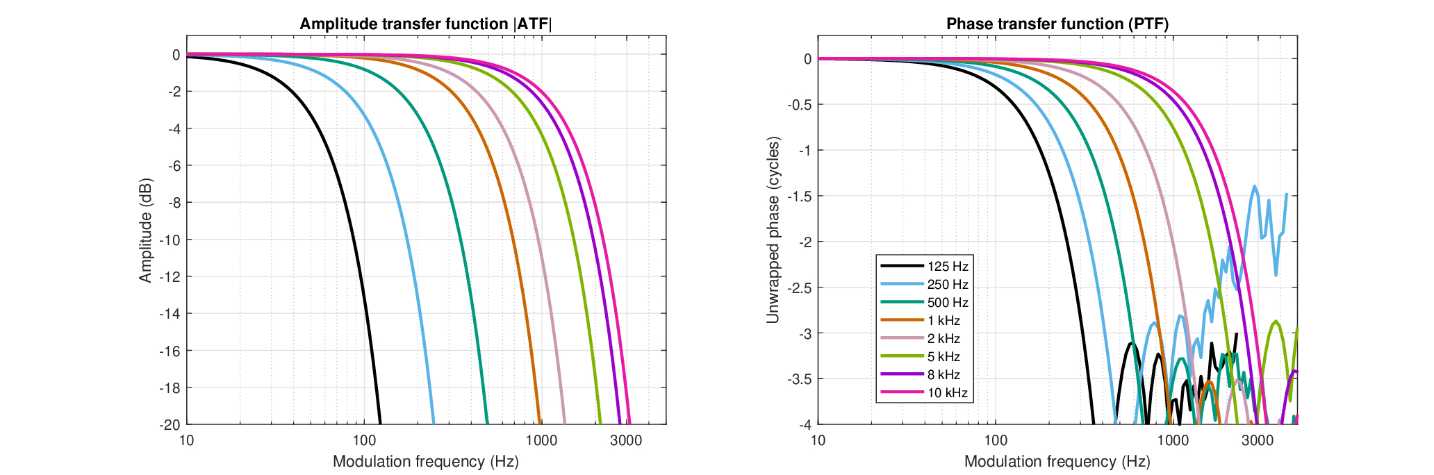
Figure 15.1: The estimated amplitude transfer function (ATF, left) and (unwrapped) phase transfer function (PTF, right) of the human auditory system (Eq. §13.25), using the parameters found in §11 and low-frequency corrections from §12.5.

Several signal types are displayed in Figure 15.2 with and without the effect of the estimated auditory ATF¹⁴². The responses were obtained by generating a complex temporal envelope and multiplying it in the frequency domain with the ATF¹⁴³. Critically, the negative frequencies of the modulation domain were retained in sound processing. The most coherent and narrowest signals are also the ones that are unaffected by the defocus and by the MTF on the whole, as its low-pass cutoff is higher than half the signal bandwidth (for signals whose carrier is centered in the auditory filter). The effect of the aperture low-pass filtering is illustrated using the different signals—notably their amplitude-modulation (AM). The defocus (i.e., its quadratic phase) directly affects the signal phase and any frequency-modulated (FM) parts (see caption in Figure 15.2 for further details). Both the narrowband noise and the AM-FM signal were deliberately designed to have relatively broadband spectra, so to emphasize the dispersive effect. In all cases but the pure tone, it is the author's impression that the defocused version may be considered less sharp than the unprocessed versions, although the effect is not the same in the different cases. The narrowband noise sounds narrower and with less low-frequency energy, which raises the perceived pitch of the filtered noise. The speech sample sounds duller, but the effect is subtle with the neural group-delay dispersion value obtained. The FM sound is made duller after filtering, and its pitch is pushed both lower and higher than the pitch of the unfiltered version. However, to simulate a more correct auditory defocusing blur may require tweaking of the parameters (neural dispersion, temporal aperture, or filter bandwidth) and more importantly, to apply nonuniform sampling that resembles adaptive neural spiking and that captures the low-pass filtering and decohering effects that it may have after repeated resampling and downsampling (§14.8).

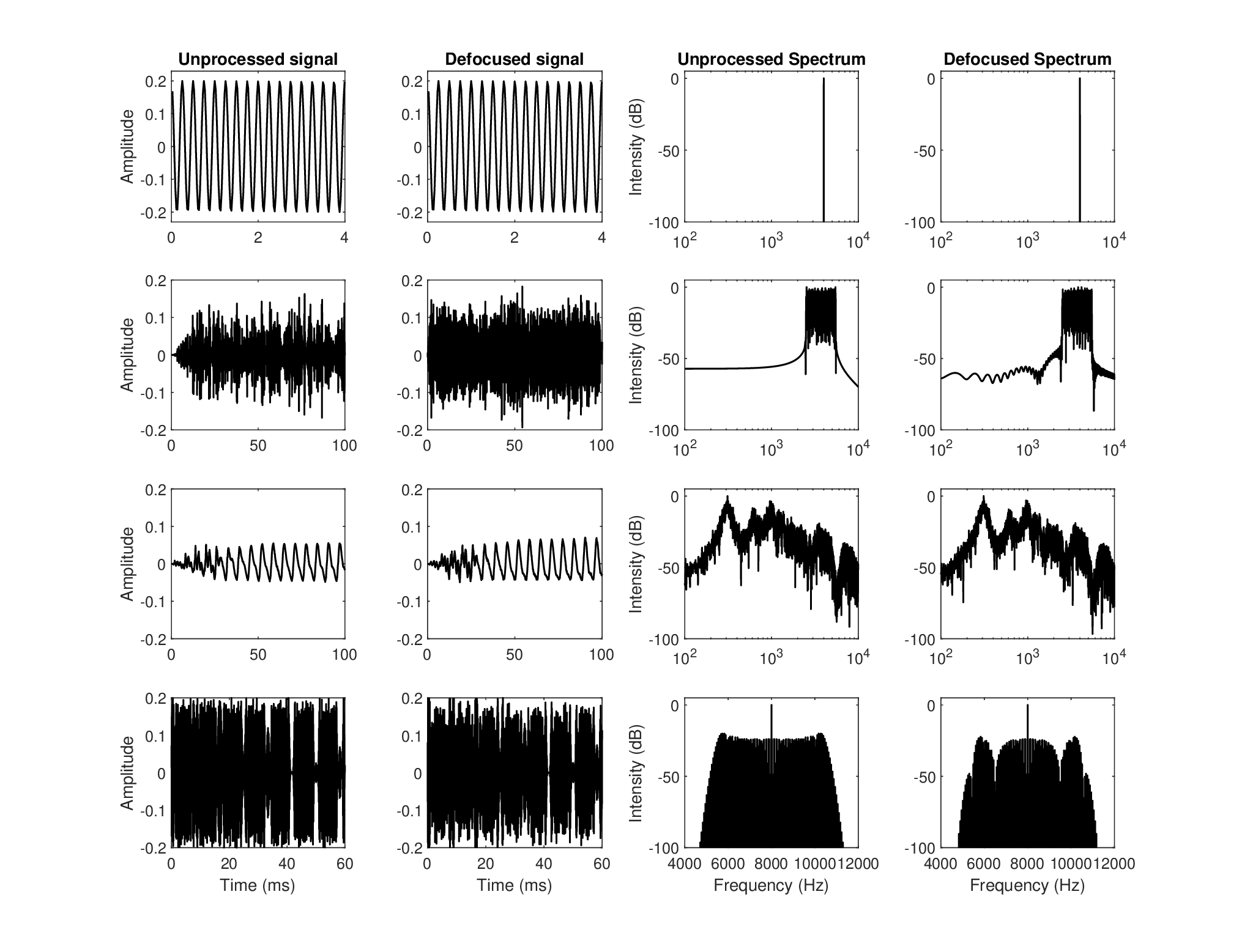
Figure 15.2: The effect of the auditory defocus on four signals of different modulation spectra and levels of coherence. Each row corresponds to a signal type, where the leftmost plot is the unprocessed time signal, the second from the left is the defocused time signal obtained by multiplying its modulation spectrum with the complex ATF (see Figure 15.1), the third is the power spectrum of the unprocessed signal and the rightmost plot is the power spectrum of the defocused signal. The first row is a 4 kHz pure tone, which is unaffected by the modulation filter. The second row is a rectangular-shaped narrowband noise centered at 4 kHz with 3 kHz total bandwidth. The processed and unprocessed sounds were RMS equalized to make their loudness comparable. The audible effect of the defocus filter is subtle, as it slightly lowers the pitch of the noise, and it is caused by both the aperture and quadratic phase. The third row is taken from a 2 s long male speech recording in an audiometric booth (only the first 100 ms are displayed) that was bandpass-filtered around seven octave bands (125–4000 Hz, 4-order Butterworth, bandwidth equal to the equivalent rectangular bandwidth (ERB) (Eq. §11.17) (Glasberg and Moore, 1990). The unprocessed version was obtained by using Hilbert envelope and phase as a complex envelope to modulate a pure tone carrier in the respective octave band and the total signal is the summation of all seven bands. The defocused version was the same, but the complex envelope was filtered in the modulation frequency domain by the ATF before modulating the carrier. The audible effect was not dominated by the quadratic phase itself, but rather by the aperture, which results in a thinner sound. The last row is of a strongly modulated 8 kHz carrier, whose AM-FM envelope is: \(1+\sin\left[2\pi 50t + 40\cos(2\pi 60t)\right]\). Once again, the audible effect is subtle and makes the defocused sound slightly muffled and lower-pitched, although this time it was caused mainly by the quadratic phase. Refer to the audio demo directory /Figure 15.2 - auditory defocus/ to hear the corresponding examples.

It appears that the auditory defocus tends to interact with sounds that are clearly broadband. When they are not resolved to narrowband filters, these sounds potentially contain high modulation frequencies that may be affected either by the low-pass amplitude response or by the phase of the ATF. The narrowband noise In Figure 15.2 is an example for such a sound, whose random variations cause instantaneous phase changes that map to very high nonstationary FM rates.

The prominence of defocus in listening to realistic sound environments is unknown at present. The most useful portion of the (real) modulation spectrum of (anechoic) speech is well-contained below 16 Hz (Drullman et al., 1994a) mostly for consonants, whereas temporal envelope information for vowels was mostly contained below 50 Hz (Shannon et al., 1995). Using the estimated auditory dispersion parameters from §11, such a modulation spectrum is unlikely to be strongly affected by group-velocity dispersion alone, which may have a larger effect on the FM parts of speech in case they can be associated with higher instantaneous frequencies. This conclusion is somewhat supported by the crudely processed speech example of Figure 15.2, which disclosed only a subtle blur compared to the unprocessed version. Nevertheless, the analysis in the final chapters of this work will suggest that the role of defocus is greater than initially may appear from the examples that were given above.

15.6 The temporal resolution of the auditory system

15.6.1 Temporal acuity

One of the most basic aspects of any imaging system is its resolving power, which quantifies the smallest detail that can be imaged distinctly from adjacent details. In spatial imaging, it is intuitively conveyed by the point spread function, which converts a point in the object plane to a disc with a blurred circumference in the image plane. The size of the disc is minimal when the system is in sharp focus and with no aberrations, as it is only constrained by the blurring effect of diffraction. An analogous effect is obtained using the impulse response function in temporal imaging, only that the limiting effect is caused by group-velocity dispersion instead of diffraction. Using the estimated system parameters, it is possible to use the impulse response function of Eq. §13.20 to compute the theoretical temporal resolution values at different frequencies.

There are several established criteria in optics for imaging resolution based on two-dimensional patterns (usually assuming circular or rectangular apertures). The most famous one is the Rayleigh criterion, which is based on the image of two object points. When the center of one imaged point falls on the first zero of the diffraction pattern (an Airy disc) of the second point, the two points are just about resolved (Rayleigh, 1879a; Goodman, 2017; pp. 216–219; §4.2.2). There is no standard criterion in temporal imaging, although Kolner (1994a) suggested one for a system with a rectangular aperture in sharp focus. In analogy to spatial imaging, he equated the location of first zero of the corresponding impulse response sinc function to the spacing required for resolving two impulses.

As the present work employs a Gaussian aperture shape—an unphysical shape that has no zeros, but is convenient to work with analytically and appears to correspond to the auditory pupil shape—the criterion here will be somewhat more arbitrary. We shall consider a sequence of two impulses as resolved if their responses intersect at the half-maximum intensity. Using the auditory system parameters found in §11 and the generalized (defocused) impulse response for a Gaussian aperture (Eq. §13.20), the resolution at different spectral bands can be readily obtained by using an input of the form \(\delta(-d/2) + \delta(d/2)\), for two pulses separated by a gap of \(d\) seconds, measured between their peaks. The gap duration can be calculated by convolving the impulse response with a delta function and finding the time \(d/2\) at which the respective intensity drops to a quarter of the maximum. The two incoherent pulses then intersect at half the maximum level. After some algebraic manipulation, we obtain the gap duration:

\[ d = v T_a\sqrt{\left(\frac{16\ln2}{T_a^2}\right)^2 + \left(\frac{1}{u} + \frac{1}{v}+ \frac{1}{s} \right)^2 } \]

(15.1)

In order to obtain the intensity response for the incoherent case, the response to each pulse was squared independently (Eq. §13.48): \(I = I(-d/2) + I(d/2)\) (black curves in Figure 15.3). In the coherent case (Eq. §13.46), the summation preceded the squaring: \(I = [a(-d/2) + a(d/2)]^2\), which is displayed in blue dashed lines of Figure 15.3.

As delta impulses are incoherent by definition, the coherent responses of Figure 15.3 are shown more for academic interest, although short Gabor pulses produce very similar results (see §F). The coherent pulses give rise to visible interference (fast oscillations) in the final intensity pattern, which does not match known auditory responses. These oscillations disappear upon increasing the gap \(d\), so that \(1.1d\) produces a more visible gap in the interference pattern, which almost vanishes completely at \(1.4d\) (some oscillations are visible in the trough). The incoherent pulses produce smooth responses that are more easily resolved using the chosen criterion, which is also how the resolution limits were determined. The response was extended up to 10 kHz, but above this frequency the estimates of the cochlear dispersion could not be trusted (see Figure §11.6).

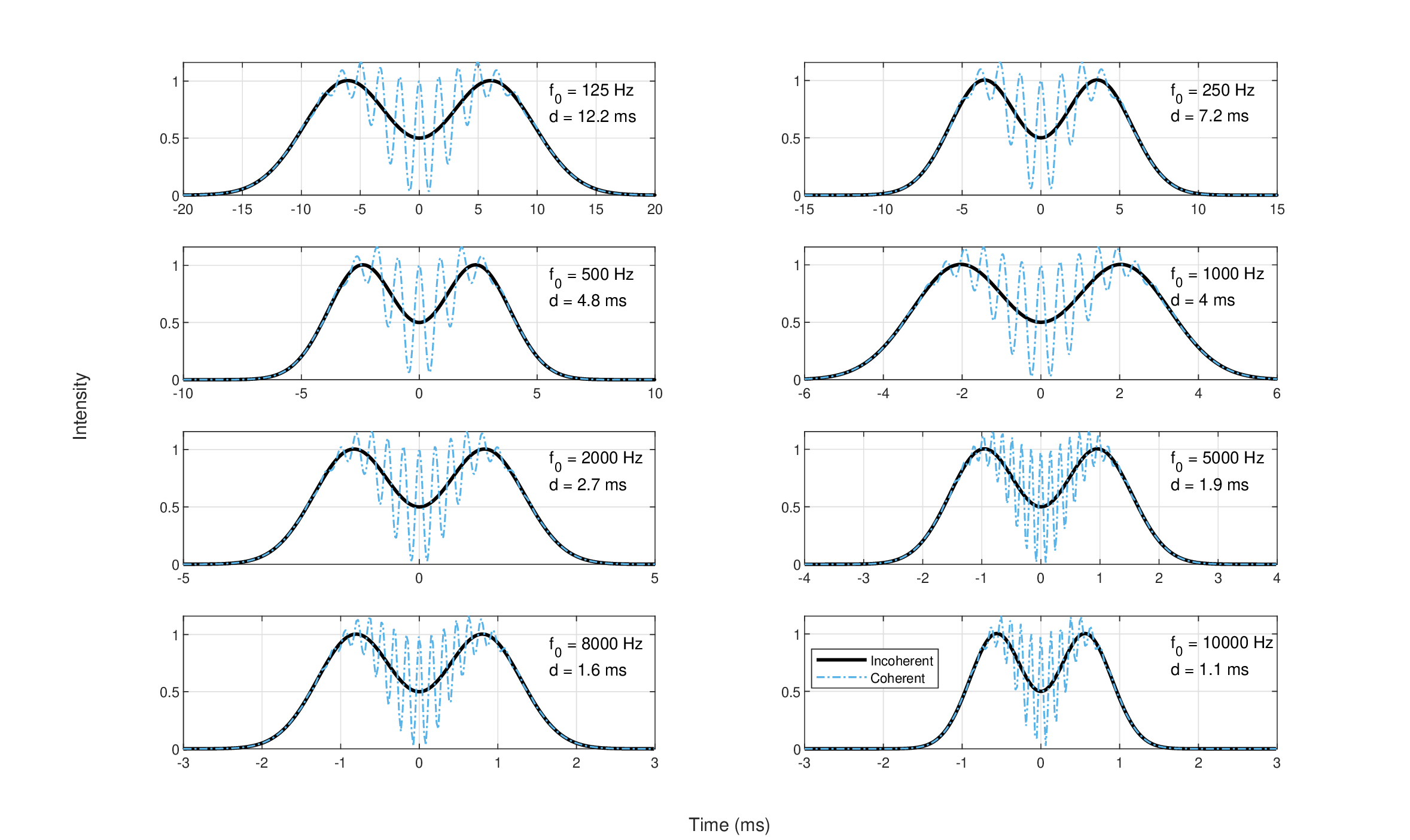
Figure 15.3: The temporal resolution of two consecutive impulses spaced by \(d\) milliseconds, according to the impulse response function of Eqs. §13.20 and 15.1 and the parameters from §11. The spacing was chosen so that pulses are considered resolved when their (summed) intensity image is exactly at half of the peak value. The black solid curve shows the incoherent pulse response. The blue dash-dot curves show the “coherent impulse responses” as a demonstration of the effect of the phase term in the defocused impulse response function. The oscillations are a result of interference, which subsides when the gap is increased.

The results in Figure 15.3 represent the output of a single auditory channel and should be compared to narrowband temporal acuity data from literature, if available. In auditory research, temporal acuity assessment and definition is challenged by the fact that multiple cues (e.g., spectral, intensity) can account for just-noticeable differences between stimuli. Therefore, different methods have been devised to obtain specific types of acuity, which are not always consistent with each other (Moore, 2013; pp. 169–202). As a rule of thumb, the auditory system is able to resolve 2–3 ms (Moore, 2013; p. 200), which corresponds well only to the obtained resolution at 2 kHz (2.7 ms) and maybe at 4 and 8 kHz (1.8 and 1.6 ms, respectively) and 1 kHz (4 ms). At low frequencies, the resolution drops (12.2 ms at 125 Hz, 7.2 ms at 250 Hz, and 4.8 ms at 500 Hz), but less so than it would have dropped had the temporal aperture remained uncorrected (i.e., if we let it be unphysically long; see §12.5.2). The 4 and 8 kHz predictions are a bit shorter than the data we obtained using Gabor pulses (see §E.2.2), which had a median acuity of 2.3–3.4 ms at 6 kHz, and 2.8–4.2 ms at 8 kHz, with the two best performing subjects having 1.8–2.7 ms and 2.1–4 ms, respectively. The two lowest frequencies as well as frequencies above 8 kHz are particularly susceptible to errors, because of greater uncertainty in the dispersion parameters and temporal aperture¹⁴⁴. Such frequency dependence of the temporal resolution has usually not been observed in past studies that employed narrowband noise (Green, 1973; Eddins et al., 1992; e.g.,][), but values as short as obtained here at high frequencies are typical with broadband stimuli (e.g., Ronken, 1971). However, gap detection (\(>\) 50% threshold) using sinusoidal tones in (Shailer and Moore, 1987; Figures 2–3) was 2–5.5 ms at 400 Hz, 2.5–3.5 ms at 1000 Hz, compared to predicted gap thresholds of 4.1 ms (not plotted) and 3.6 ms, respectively.

Implicit to this discussion is that the built-in neural sampling of the auditory system can deal with arbitrarily proximate pulses. This is probably true for broadband sounds that stimulate multiple channels along the cochlea, but may be a stretch for narrowband sounds, whose response depends on fewer fibers¹⁴⁵. At least in the bandwidth for which data are available, this assumption appears to be met.

This gap detection computation was based on a Gaussian-shaped pupil function, which appears to be approximately valid (§12.5). However, we do not know the actual pupil function shape in humans, which may eventually alter these estimates to some extent.

15.6.2 Envelope acuity

While the temporal acuity as quantified above defines the shortest sound feature that can be resolved within a channel, such a fine resolution of 2–3 ms is not generally found in continuous sound, where the acuity tends to significantly degrade. This was measured in Experiments 4 and 5 in §E with click trains that included 8 or 9 clicks, to reduce the onset effect and induce some pattern predictability in the listener. When these short events are interpreted as modulations, they suggest a drop in the instantaneous modulation rate from 300–600 Hz to 60–100 Hz. This suggests that the bandwidth of the various psychoacoustic TMTFs may not necessarily reflect the fidelity as it relates to the specific contents of the temporal and spectral envelopes.

Several studies can attest to this assertion. For example, the discrimination between amplitude-modulation frequencies has been tested a few times with tonal, narrowband noise, and broadband noise carriers (e.g., Miller and Taylor, 1948; Buus, 1983; Formby, 1985; Hanna, 1992; Lee, 1994; Lemanska et al., 2002). Roughly, these measurements reveal that the discrimination is fairly good (about 1–2 Hz) for low modulation frequencies (below 20 Hz) and gets gradually worse at high modulation frequencies (approximately 20 Hz for 150 Hz modulation, for unresolved modulations). This repeats for different carrier types and frequencies and does not vary much between listeners. Such findings support the model of an auditory modulation filter bank that has broadly tuned bandpass filters, which get broader at higher modulation frequencies, similar to the critical bands in the audio domain (Dau et al., 1997a; Dau et al., 1997b; Ewert and Dau, 2000; Moore et al., 2009). A more recent study demonstrated how listeners are not particularly sensitive to irregularities in the temporal envelope, which were superimposed at lower frequencies than the regular AM frequency under test (Moore et al., 2019). The results of this experiment suggest that fluctuations in the instantaneous modulation frequency can go unnoticed by many listeners, who perceive a relatively coarse-grained version of the envelope. However, the individual variation in this experiment was large.

Since we defined blur earlier as a change in the contents of the temporal, and hence in the spectral envelope, then these studies suggest that the system may not be particularly sensitive to blur in the modulation domain, at least in conditions of continuous sounds, as opposed to onsets or impulsive sound. In a way, this perception may represent a form of internal blur that corresponds to a tolerance that the auditory system has to different complex stimuli.

15.7 Polychromatic images

So far, the discussion and analysis of the auditory temporal images were done within a single narrowband channel. However, the modulation in real acoustic objects tends to affect multiple vibrational modes and is rarely limited to narrowband vibrations (single modes). For example, during a drum roll, the modes of vibrations of the drum get excited together—they are comodulated—in a unique pattern of sound. More complex sounds such as speech also show high correlation across the spectrum in different modulation frequency bands—especially below 4–6 Hz (Crouzet and Ainsworth, 2001). The analogous optical situation is of an object that is lit by white light, whose spatial modulation spectra—one spectrum per color channel—are highly correlated as a result of being reflected from the same object, whose geometry affects all wavelengths nearly equally. The imaged object is then sensed as a superposition of very similar images of different primary colors, which can be processed by the corresponding cone photoreceptors (Figures 15.4 and 15.5). Importantly, the images created by the photoreceptor channels spatially overlap in a way that facilitates the perceptual reconstruction of the original object. In analogy, we would expect that the broadband auditory image would stem from a perceptual re-synthesis of temporally modulated narrowband images in different channels, which represent the acoustic object response as a whole. This across-channel broadband image is referred to as polychromatic—an adjective that distinguishes it from a mere broadband sound, for which the identity of the constituent monochromatic channels may be inconsequential .

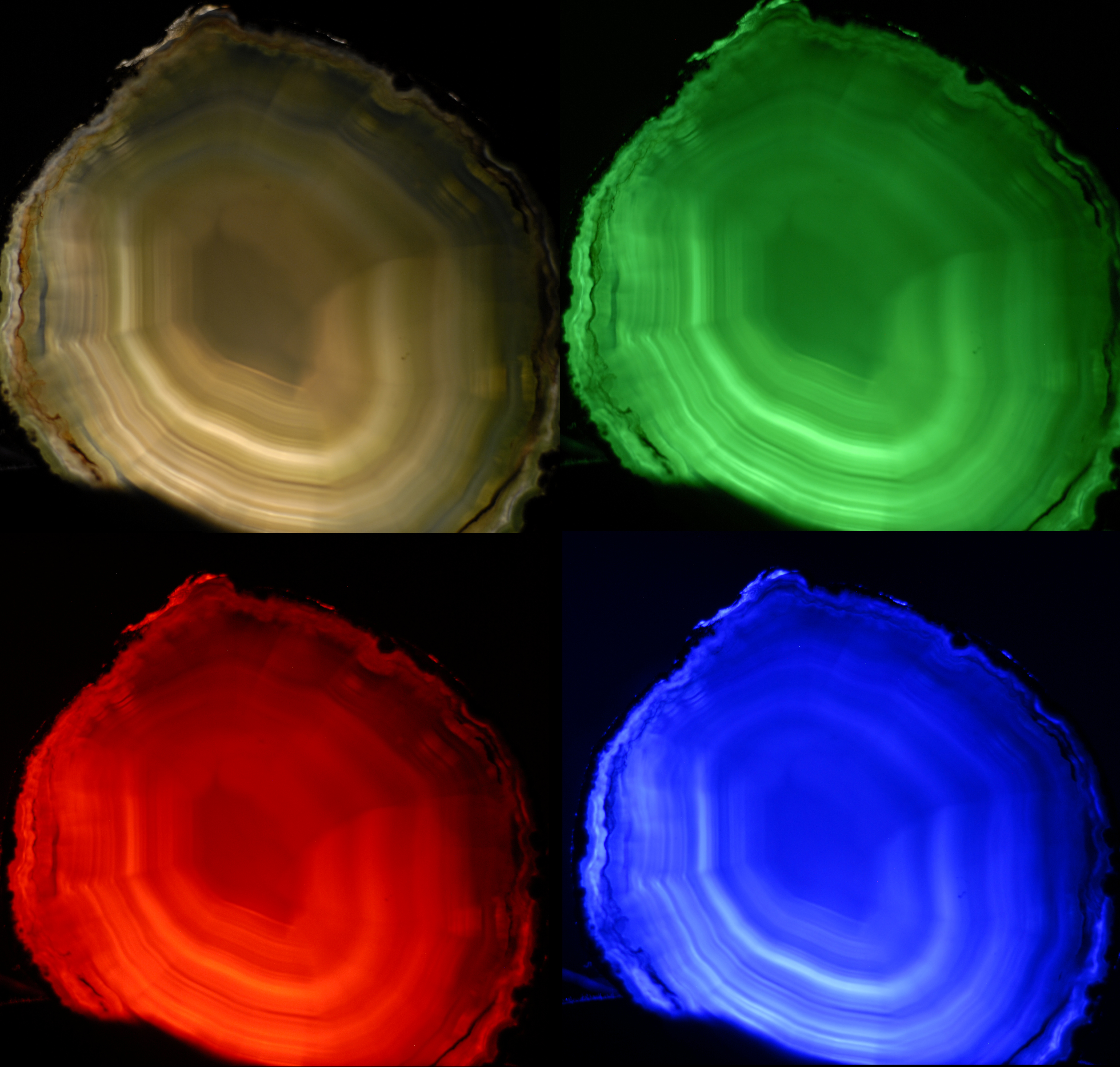
Figure 15.4: Four images of a polished agate rock that is back-lit by an LED incoherent light source with variable colors. The top-left image is illuminated with white light (full spectrum) that produces the polychromatic image. The other three images are all monochromatic. Different details of the agate surface are emphasized under each light. More technical details about the LED sources are in Figure §8.3.

That the auditory system indeed combines across-channel modulation information as generated by common events has been repeatedly demonstrated in several effects—most famously, through the phenomenon of comodulation masking release (CMR; Hall et al., 1984). Normally, when a target tone is embedded in unmodulated broadband noise, its detection threshold increases as the noise occupies more of their shared bandwidth within a single auditory channel. The strength of this masking effect depends on the noise bandwidth as long as it is within the channel bandwidth, but is unaffected by noise components that are outside of the channel. However, if the noise is extended beyond the channel bandwidth and is also amplitude-modulated (not necessarily sinusoidally), then the masking effect decreases—information from adjacent and remote noise bands is used by the auditory system to release the target from the masking effect of the noise (see top plots in Figure 15.6). The effect is robust and has been shown to yield up to 10–20 dB in release from masking, depending on the specific variation (Verhey et al., 2003; Moore, 2013; pp. 102–108). The effect is also more or less frequency-independent, as long as the bandwidth of the noise is scaled with reference to the auditory filter bandwidth of the target (Haggard et al., 1990).

CMR has been interpreted as a form of pattern recognition and comparison across different bands of the signal, which is representative of real-world regularities of sounds (e.g., Hall et al., 1984; Nelken et al., 1999). As such, it is also considered an important grouping cue in auditory scene analysis (Bregman, 1990; pp. 320–325), which is effective as long as the different comodulated bands are temporally synchronized (or “coherent”, in the standard psychoacoustic jargon, §7.2.4) (Christiansen and Oxenham, 2014). In stream formation, temporal coherence (of the envelopes) can act as a strong grouping cue that binds across-frequency synchronized tones, but not asynchronous tones whose onsets do not coincide (Elhilali et al., 2009).

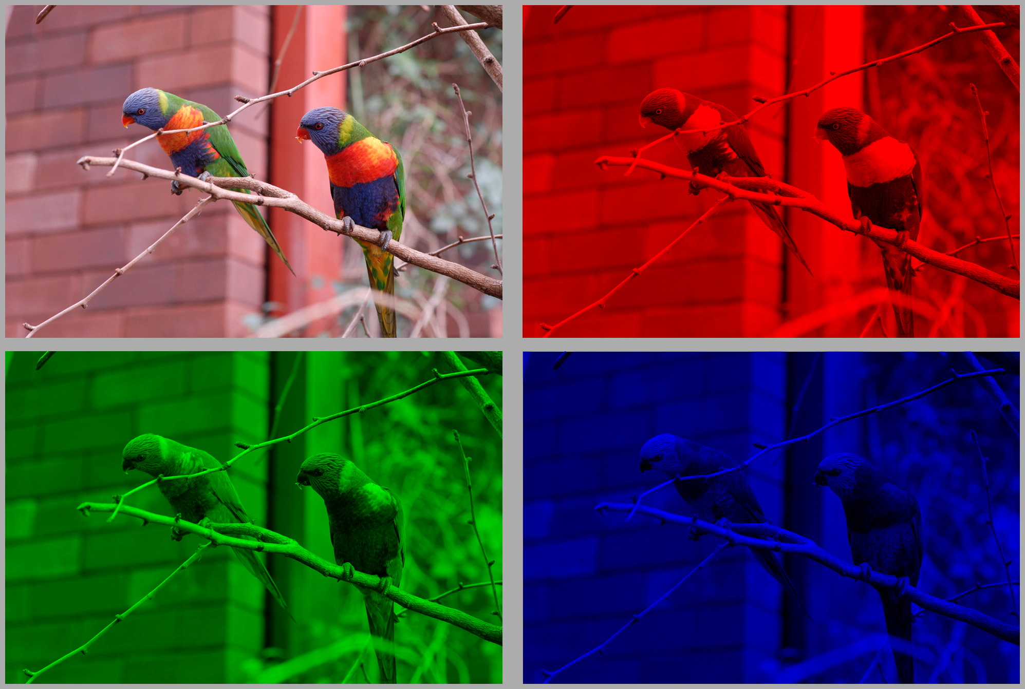
Figure 15.5: An illustration of a polychromatic image decomposed into three monochromatic color channels. The image is a spatial modulation pattern carried by incoherent broadband light, which is detected in three narrowband channels in the retina by red, green, and blue photoreceptors (long, medium, and short wavelength cones, respectively). The three monochromatic images are very similar, but some object details are not observable in all of them. For example, the birds' eyes appear to be almost uniform in blue light, whereas the existence of the iris and pupil can be seen most clearly in red and much less clearly in green.

There has been only one physiological demonstration of CMR at early processing stages (Pressnitzer et al., 2001). Spiking pattern correlates of CMR were found in the guinea pig anteroventral cochlear nucleus (AVCN) units—mainly of the primary-like and chopper-T types. In order for this effect to work, low-level integration is required that relies on the modulated masker in different channels to be in phase. The authors modeled the results using a multipolar broadband unit that receives excitatory off-frequency inputs, which in turn inhibits a narrowband in-channel unit—inhibition that results in masking release. The existence of a broadband processing stage is supported also by psychoacoustic data, which ruled out a model of across-channel comparison of the different narrowband envelopes (Doleschal and Verhey, 2020). Furthermore, the CMR model of Pressnitzer et al. (2001) was successfully used to demonstrate how across-channel information may be advantageous in consonant identification under different conditions (i.e., in noise or when the temporal fine structure was severely degraded; Viswanathan et al., 2022).

Other effects exist that demonstrate the polychromatic auditory image primacy over spectral mechanisms, as the system prioritizes temporal cues of multiband signals at the apparent expense of unmodulated narrowband target signals. For example, in modulation discrimination interference (MDI), an amplitude- or frequency-modulated masker causes the decrease in detection sensitivity of a similarly modulated target at a distant channel (Figure 15.6, bottom right) (Yost et al., 1989; Wilson et al., 1990; Cohen and Chen, 1992). Thus, the modulated target cannot be easily heard as being separate from the masker. However, FM elicits a more limited MDI effect that does not always provide sufficient resolution across channels and modulation patterns, at least at high modulation frequencies (e.g., Lyzenga and Moore, 2005). Profile analysis is another phenomenon, whereby the detection of a level change of one of the components of a multicomponent masker depends on the entire across-frequency profile of the masker (Figure 15.6, bottom left) (Spiegel et al., 1981). The detection of a single-component target improves when the masker has known frequencies compared to when there is some uncertainty in its component frequencies. The spectral profile is often modeled as spectral modulation (e.g., Chi et al., 1999).

It may be argued that in all three effects mentioned—CMR, MDI, and profile analysis—the experimenters' designation of signal and noise (or target and masker) is incongruent with what the auditory system determines. Once the system identifies a potential across-frequency image, it attempts to optimize it as a whole, rather than as a loose collection of monochromatic images.

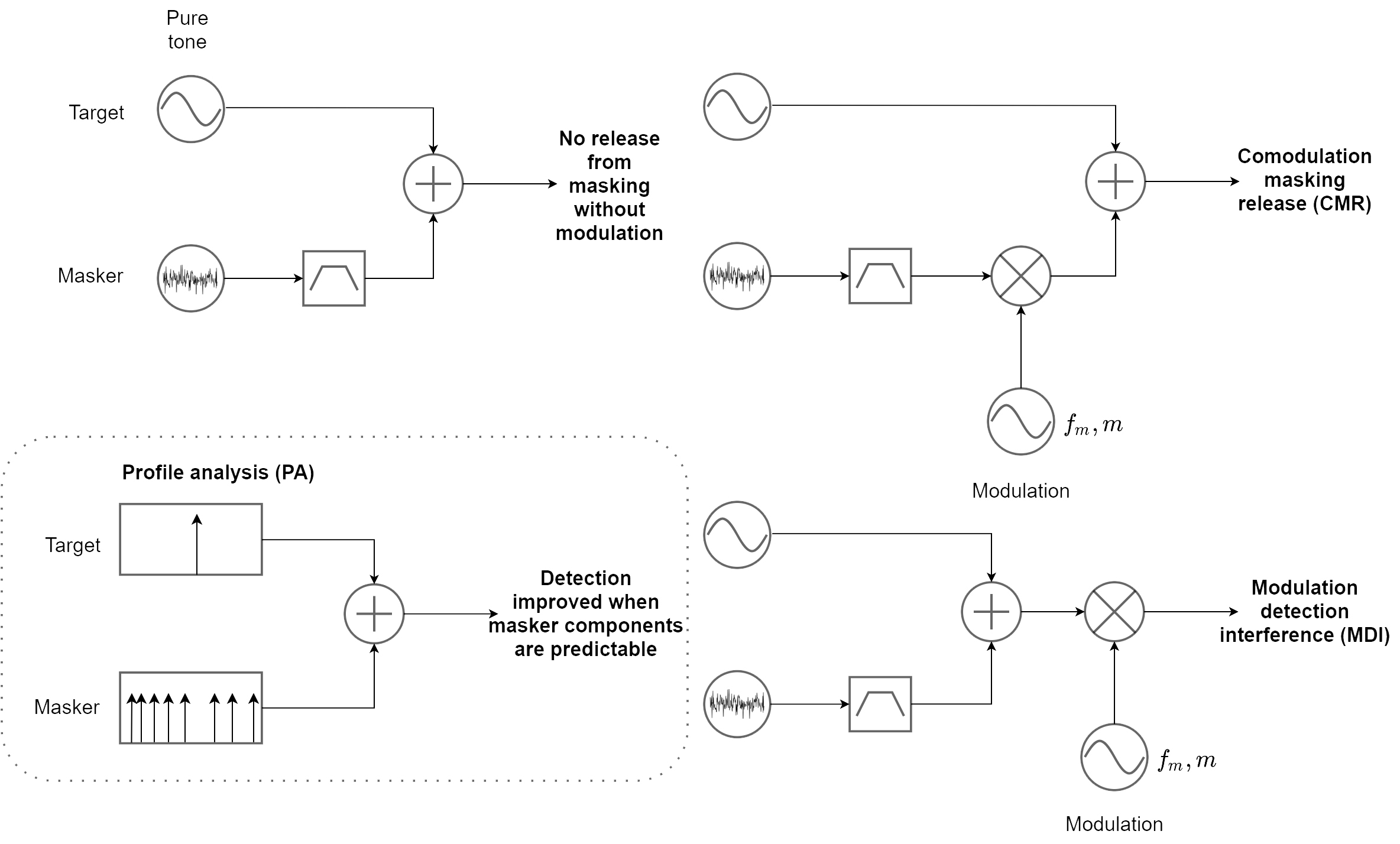
Figure 15.6: Three psychoacoustic paradigms that entail broadband information integration, beyond a single auditory channel. On the top left, the standard paradigm is shown of a target tone in masking noise. The bandpass filter symbol indicates that the masker bandwidth is a parameter in these experiments. Modulation is indicated with a sinusoidal source of frequency \(f_m\) and depth \(m\), which multiplies the noise or signal and noise. Multiplication is indicated by the mixer (cross sign).

The importance of the polychromatic representation in an ensemble of monochromatic channels may be gleaned from a study in cochlear implant processing by Oxenham and Kreft (2014). The authors showed how, unlike normal-hearing listeners, the speech-in-noise performance was identical for the cochlear-implant users regardless of the type of masker used: broadband Gaussian noise with random fluctuations, broadband tone complex with the same spectral envelope as the broadband noise, and the same tone complex with the superimposed modulation of the Gaussian noise. It was found that this undifferentiated pattern is not caused by insensitivity to temporal fluctuations, but rather by spectral smoothing, as the cross talk between the implant electrodes within the cochlea causes the different channel envelopes to mix across the spectrum. This was shown from speech intelligibility scores of normal-hearing listeners, who could no longer take advantage of the fluctuation difference between masker types, after the temporal envelopes extracted from 16 channels were summed and identically imposed on all 16 channels.

These phenomena and others may all attest to the image dominance, where modulation is involved, compared to unmodulated isolated sounds¹⁴⁶. The CMR effect originally appeared to violate the critical band theory, which predicts that only information within auditory filters should be fused. However, by analogy to vision, this effect may be predicable if the auditory system “overlays” multiple monochromatic images to produce a single polychromatic image, or a fused or coherent stream, according to auditory scene analysis. MDI too is consistent with the system trying to form auditory images (“objects” in Yost et al., 1989) from a common acoustic source. Unlike vision that has its three monochromatic detectors interwoven in the same spatial array on the retina, overlaying the auditory imaging has to be done in time. Such a mechanism has been discussed at length with regards to periodicity in the inferior colliculus (periodotopy; Langner, 2015), which is nevertheless more restricted than general modulation patterns that are not necessarily periodic.

As a final note, it should be emphasized that some broadband sounds may not be amenable to representation as polychromatic images, if they vary across channels and time in an independent manner across channels.

15.8 Pitch as an image

It is worth dwelling briefly on tones and pitch, which have captured the spotlight of auditory research throughout most of its history in one form or another. This section is not concerned directly with how the pitch is determined within the auditory system as a function of the stimulus properties, or in which frequency range each of the pitch types exists. It does, however, attempt to illustrate how the idealized auditory image is related to this standard stimulus family, in order to elucidate interrelated aspects in the pitch and imaging theories. Different pitch types are analyzed using three spectra—of the carrier (through a filter bank), the envelope (or baseband), and the power spectrum that contains the same information as the broadband autocorrelation. The last two spectra require nonlinearity to either demodulate the signal, or generate harmonic distortion that produces the square term that explicitly reveals the fundamental.

It should be noted that while the information required to give rise to monaural pitch is available already at the level of the inferior colliculus (IC), pitch perception is most likely generated in the auditory cortex after appropriate coding transformation (Plack et al., 2014). The early availability appears to hold also more generally to nonstationary pitch, such as the fundamental frequency in speech, which is tracked at the level of the IC (Forte et al., 2017). Inharmonic complex tone pitch and binaural pitch, though, may require information that is derived after some processing that may take place at a higher level than the IC as well (Gockel et al., 2011). Therefore, these general results suggest that an image that appears at the IC can be used to infer some properties of pitch, even if it is produced and perceived further downstream. We shall use employ our own auditory image concept loosely here to relate directly to the physical stimulus, but also link it to the psychoacoustic percept, which is assumed to be directly derived from the image, at least for the simple examples used below. Cartoon spectra of four of the most common monaural pitch types are displayed in Figure 15.7 and are described below in some detail.

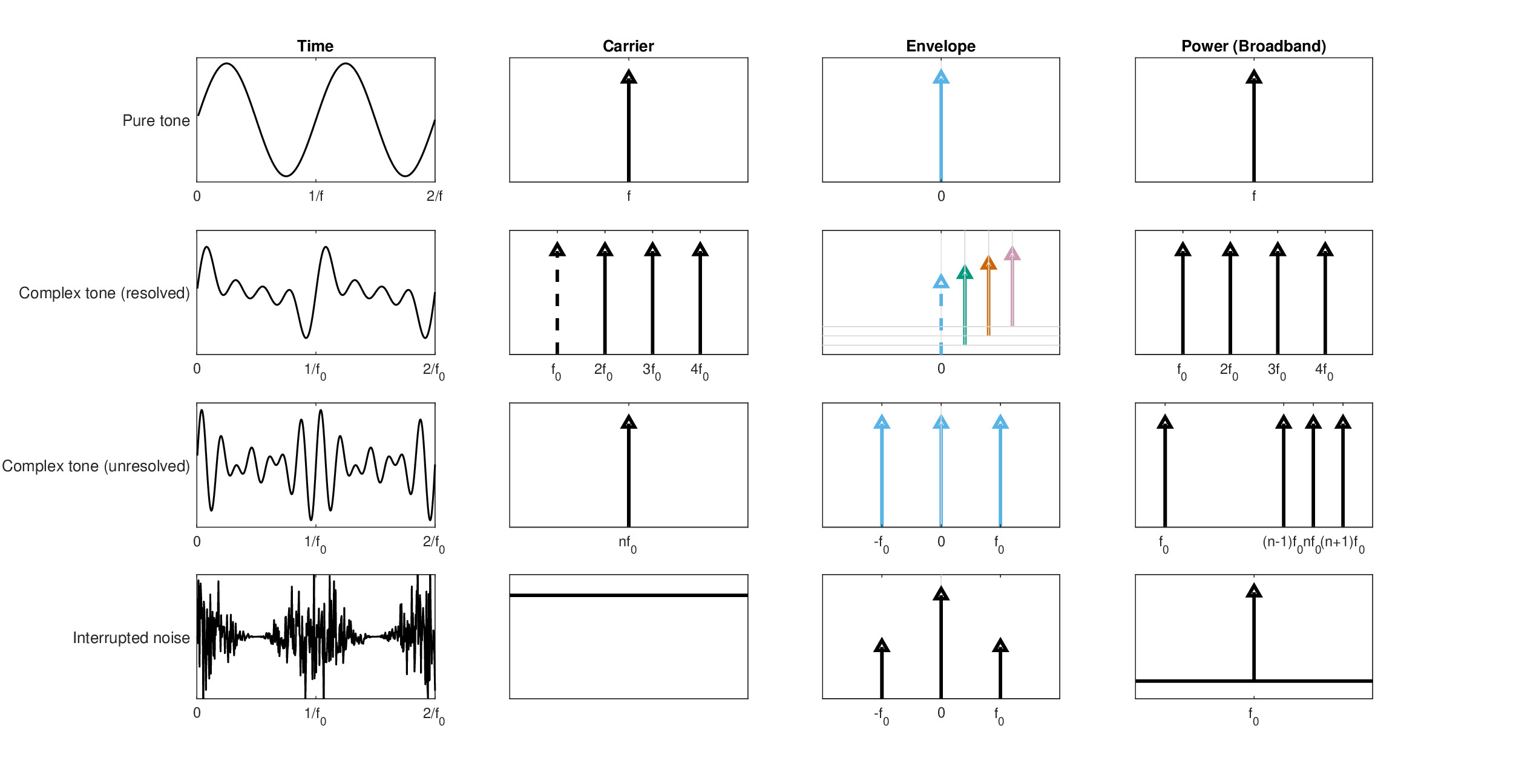
Figure 15.7: Cartoon spectra of four stimuli that elicit four common types of monaural pitch. Two periods of each time signal appear on the left along with three different spectra on the right. On the second column is the filter-bank spectrum that can identify the carrier. On the third column is the modulation spectrum, which is the baseband spectrum of the filter output after demodulation. This is where the monochromatic object and image reside. Finally, on the rightmost column is the power spectrum, which has to follow some nonlinearity (e.g., half-wave rectification and squaring), although here it excludes additional harmonic distortion products, for clarity. On the top row is a pure tone, which has a single component in all three spectra that makes its image degenerate. On the second row is a complex tone, whose components are individually resolved in one filter each, with its fundamental frequency \(f_0\) intact, or missing (dashed spectral lines). Its envelope spectrum contains only the DC component in each channel, which is associated with a harmonic, and is thus analogous to a polychromatic image. The power spectrum contains \(f_0\), whether it appears in the stimulus or not. On the third row is an unresolved complex tone, whose components are analyzed by a single filter, where it appears like a single component. Its ideal modulation image contains all three components, whereas the power spectrum also contains the missing fundamental (although it is heard more faintly). On the bottom row, a form of periodicity pitch—interrupted noise—is produced by amplitude-modulating white noise, which assumes some pitch if it is fast enough. The power spectrum can reveal the modulation period that is seen in the envelope spectrum, on top of the spectral distribution of the noise itself.

The pure tone is probably the most widely used and abused stimulus in all of acoustics. But what does it entail within the temporal imaging framework? As the pure tone has a real and constant envelope, its ideal image also has a constant envelope with an arbitrary magnification (gain). We hear the constant envelope along with a uniform pitch percept without perceiving the tonal oscillations. Therefore, this is an intensity image, rather than an amplitude image. Such an image is completely static (or “stable” according to Patterson et al., 1992), because it is time-invariant. It is contrasted with arbitrary acoustic objects that have time-dependent amplitude and phase functions that give rise to complex envelopes. Therefore, a pure tone is also coherent in two senses. In the classical sense, a pure tone is obtained from a perfectly (temporally) coherent signal that can always interfere with itself¹⁴⁷. In the auditory jargon usage of coherence, as the pure tone has no beginning and no end, it is always coherent in the envelope domain as well, whose spectrum contains only a single line at zero (DC). Therefore, we can think of the pure tone as a degenerate image¹⁴⁸. In analogy to vision, such an image would correspond to a monochromatic dot object that is fixed in space right on the optical axis and is projected as a still (spread) point at the center of the fovea.

Complex tones refer to series of pure tones with fixed spacing between their frequency components and common onsets and offsets. The series is usually harmonic, which means that the spacing between the component frequencies follows an integer ratio. It is possible to generate harmonic series so that each tone is resolved in its own dedicated auditory channel, which prevents audible beating between components from taking place. This gives rise to a series of degenerate images. But, the auditory system also extracts the periodicity of the harmonic series, which in this case corresponds to the lowest-frequency spectral line in its broadband power spectrum. Thus, while more complex, this image is still static and has a distinct pitch that corresponds to the fundamental frequency—the spacing between the components. Additionally, because of the integer ratios between the harmonics and the frequency spacing, it is also a degenerate image, but in a different sense: the fundamental frequency of the harmonic series coincides with the periodicity from the power spectrum. This gives rise to the famous missing fundamental effect, when the harmonic series excludes the fundamental—the perception that the pitch corresponds to the fundamental even when it is absent from the stimulus. There is no complete analog to this image in vision, but the periodicity spectrum is analogous to a grating, whereas each component corresponds to a color. However, we cannot represent their harmonic relations visually¹⁴⁹\(^,\)¹⁵⁰.

For limited harmonic series with small frequency spacing and only few components, the harmonics may not be resolvable, so they are analyzed mainly within a single channel. In general, such series can be mathematically represented as interference or beating patterns that modulate a carrier. It means that the envelope spectrum contains at least two components (i.e., a DC component at zero and at the beating frequency), whereas the carrier domain has only one. The broadband power spectrum again shows the fundamental that corresponds to a residual pitch. However, the image in itself—the temporal envelope—is monochromatic. This pitch usually produces a more faint pitch sensation than other pitch types.

Interrupted pitch is another interesting type of pitch that is produced strictly by modulating broadband noise that does not contain any tonal information. Thus, it has no distinct components in its carrier spectrum. It has nontrivial components only in its envelope and power spectra.

The objects of more realistic sounds are generally not time invariant, so they give rise to nondegenerate images. These images may have variable carriers that are more intuitively expressed using frequency modulation than using a stationary carrier spectrum with multiple components (for example, the two bottom-right plots in Figure 15.2). Realistic objects can also have nonuniform frequency spacing, which eliminates periodicity and makes the within-channel broadband envelope spectrum nonstationary as well. Complex tone objects may also be frequency-shifted—an operation that retains time-invariant carriers and envelopes in resolved channels, but produces aperiodic broadband spectra in unresolved channels (with more than two components).

Each type of pitch, therefore, reveals a different feature of the auditory system. When the corresponding spectrum or feature of the stimulus is degenerate, it elicits a stable sensation that we call pitch. Part of the multiplicity of pitch types may go back to the fact that, in general, there is no unique mathematical representation for broadband signals, so the auditory system may have had to develop ways to “corner” the signal analysis and make it sound unique by comparing information from different spectra.

Three questions can be raised following this high-level characterization of pitch. First, must all images be perceived with pitch? Second, do “pitchiness” and sharpness refer to the same underlying quality in hearing? Third, does the perception of pitch always require periodicity? According to our image definition—the scaled replica of a temporal envelope pulse—the answer is “no” to the first question, since the image appears at a more primitive processing stage than the pitch. As for the second question, the temporal auditory image refers to an arbitrary complex envelope of a single mode of the acoustic object, but the imaging condition says nothing about its duration, which is essential to elicit pitch. This situation is complex, because the perception of pitch entails sharpness. Also, increase in blur can erode the pitch of a sound, but not eliminate it. Therefore, there is a strong association between pitch and sharpness, but there are examples for pitched sounds that are not sharp (Huggins pitch is a clear one), and for sharp sounds that are not pitched (perhaps like a snappy impulse, such as a snare drum). Therefore, while it seems that the answer to this question is a cautious “no”, a more exhaustive answer probably demands further research. As for the third question, linearly frequency-modulated tones (glides) do not have a fixed pitch and they are not periodic. However, they certainly elicit a perception of pitch, albeit a dynamic one (de Cheveigné, 2005; pp. 206–207). Therefore, the answer here is negative as well.

Interestingly, the property of pitchiness, or pitch strength, is inversely proportional to the bandwidth of the signal (Fastl and Zwicker, 2007; pp. 135–148), or maybe to its coherence time that is directly dependent on the bandwidth (Eq. §8.31). So, tones have a very long coherence time, whereas broadband noise have a negligible one, and narrowband noise somewhere in between. It also indicates that the auditory system is configured to have complete incoherence only for full bandwidth inputs, which include several critical bands. The corollary is that a single channel may have residual coherence even with random narrowband noise, by virtue of its limited bandwidth. This is in line with the conclusions from literature review about apparent phase locking to broadband noise (§9.9.2) and the discussion about temporal modulation transfer functions of partially coherent signals (§13.4.5).

15.9 Higher-order monochromatic auditory aberrations

15.9.1 General considerations

Basic spatial imaging harnesses the paraxial approximation, which requires light propagation in small angles about the optical axis and perfectly spherical or planar wavefronts. In realistic optical systems, these approximations are increasingly violated the larger the light angle is and when the various optical elements are imperfect—imperfections that are collectively called aberrations. The nonideal image exhibits various aberrations that can be studied as departures from ideal imaging. It can be done through wavefront and ray analysis, by comparing the path difference of different points along the same wavefront, as it propagates in space, which should have equal optical length in aberration-free imaging. In general, all imaging systems have a certain degree of primary higher-order aberrations and the eye is no exception—something that was already recognized by Helmholtz (1909, pp. 353–376). In the design of optical systems, aberrations are eliminated or mitigated by balancing them with other aberrations in specific conditions, although this process results in the generation of yet higher-order aberrations (Mahajan, 2011).

In wave optics, the geometrical optical wavefront analysis is elaborated by the inclusion of higher-order phase effects, beyond the quadratic phase terms that characterize the diffraction integral and the lens curvature. Similarly, in deriving expressions for the time lens and group-velocity dispersive medium, the phase functions used in the theory were expanded only up to second order that implied quadratic curvature (§10), which can account for defocus and chromatic aberrations. The existence of additional phase terms that depend on higher powers of frequency or time would drive the channel response away from its ideal imaging (Bennett and Kolner, 2001). However, because the dimensionality in temporal imaging is lower than in spatial imaging, not all of the known spatial aberrations have relevant temporal analogs.

Because the auditory channels are relatively narrow and the aperture stop is very short, higher-order aberrations may be difficult to observe, or they may appear completely absent—something that reflects the paratonal approximation that is analogous to the paraxial approximation. It is not impossible that the normal functioning hearing system circumvents higher-order aberrations by having a dense spectral coverage with dedicated fine-tuned filters along the cochlea—each of which has diminishingly low aberration around its center frequency. In other words, the various auditory filters are optimal around their characteristic frequency but are overtaken by other filters away from it, off-frequency. An additional mitigating factor is that higher-order aberrations are severer for magnification values that are much different than unity \(|M| \gg 1\) or \(|M| \ll 1\) (Bennett and Kolner, 2001), whereas our system is much closer to \(M\approx1\). Finally, the defocus itself, which is a second-order aberration, may mask the smaller effects of the higher-order (third and above) aberrations. So for example, spherical aberration is symmetrical around the channel center frequency and generally results in increased blur away from the (spatial or temporal) image center, which may be masked in hearing.

To the extent that higher-order aberrations are a real concern, they may also be difficult to identify using our pupil function and, hence, the point spread function analysis (Mahajan, 2011; pp. 77–137), which we estimated only up to second order. While it was assumed for convenience that the auditory aperture is Gaussian, the single measurement that determined its shape directly, had an asymmetrical tail attached to the Gaussian from the right (the forward-time direction; §12.5). It can be expected to cause the point spread function of the system to have asymmetrical (odd) higher-order phase terms.

The implications of having higher-order phase terms can be made more concrete by closely examining the dispersive elements of the system. If the phase curvature in the filter skirts is not exactly quadratic, then various asymmetrical dispersive aberrations analogous to spatial optics may exist—coma (third-order phase term in the Taylor expansion, Eq. §10.27), and spherical aberration (fourth-order term) (Bennett and Kolner, 2001). These terms may be detrimental to perceived sound quality when the excited channel is either over-modulated (reaching high instantaneous frequencies that should be normally resolved into multiple filters), or is more simply excited off-frequency—away from its center frequency¹⁵¹. These situations entail that the auditory channel works beyond its paratonal approximation—well-beyond its center frequency, whose role is analogous to the spatial optical axis¹⁵².

There is little physiological evidence that directly indicates that the phase curvature of the cochlear filters is asymmetrical away from the characteristic frequency, or even not perfectly quadratic. In contrast, a few psychoacoustical studies may be interpreted as showing such an asymmetry. We briefly mention evidence to the former and then focus on evidence to the latter and offer another example of our own to demonstrate this effect.

15.9.2 Physiological evidence

There is mixed physiological evidence for an ideal quadratic phase response of the auditory system. In physiological recordings of frequency glides in auditory nerve fibers of the cat, the instantaneous frequency chirps were best fitted by linear functions that indicated a quadratic phase term only (Carney et al., 1999). In several instances the glides were not linear, but better fits could not be obtained using higher order regression, including those made with log frequency. Linearity in the instantaneous frequency slopes was generally observed in the barn owl as well (Wagner et al., 2009). In contrast, in impulse responses measured using different methods in the guinea pig, chinchilla, and barn owl, the slopes of the instantaneous frequency or the phase were usually linear only in part of the response, or they changed only well below the characteristic frequency (de Boer and Nuttall, 1997; Recio et al., 1997; van der Heijden and Joris, 2003; Fontaine et al., 2015). This may be indicative of some asymmetry in the phase response of these auditory channels.

It should be noted that these measurements consider the auditory system to be dispersive only within the cochlea. This necessarily includes one segment of the neural dispersion (i.e., the path between the inner hair cells and the auditory nerve), which may have a complex phase function in itself. Additionally, these measurements tend to treat the phase response (and the filtering in general) as time-invariant, which is questionable if the outer hair cells produce active phase modulation. Therefore, we shall look for more qualitative psychoacoustic evidence of higher-order aberrations, which includes the complete dispersive path.

15.9.3 Psychoacoustic evidence

If the normal auditory system has a temporal coma aberration, then it might be possible to observe its effect when a filter is excited asymmetrically (off-frequency) with an adequate modulation spectrum. With coma, point images are smeared asymmetrically to one side, which is also the reason for the name coma—it refers to the distinct comet-like smear of the affected image points in two dimensions. If a coma-free dispersive channel is completely uniform over its entire bandwidth, then, to a first approximation, its demodulated temporal image is invariant to how the envelope object is oriented about its center. Distortion is another type of aberration, which has not been considered in the temporal imaging literature, that is sensitive to the orientation about the center frequency. In spatial imaging it appears as uneven magnification of the image, so that its circumference is deformed in relation to its center, endowing the image with the familiar barrel or pin-cushion deformations. Unlike transverse chromatic aberration that also exhibits nonuniform magnification in the context of polychromatic imaging, distortion does not cause any blur within the monochromatic image. Just like the auditory spherical aberration, distortion aberration is presently impossible to estimate. However, the combined effect of these hypothetical temporal aberrations may be tested using off-frequency stimuli. Three examples were found in literature that support this idea are described below.

Direct psychoacoustic evidence that the phase curvature is not constant across the auditory channel has been provided by Oxenham and Ewert (2005) and Wojtczak and Oxenham (2009). These studies are near replications of the curvature estimation study by Oxenham and Dau (2001a) that was described in §12.4.1. For Schroeder phase complex maskers centered on the 1, 2 and 6 kHz target tones, the threshold was minimized for a particular masking curvature, as shown previously. However, for maskers that were centered off-frequency, below the target frequency, there was no optimal curvature at 1 kHz and 2 kHz, and zero curvature at 6 kHz (Wojtczak and Oxenham, 2009), and also zero or not well-defined optimal curvature at 2 kHz in Oxenham and Ewert (2005) with a slightly different stimulus. In these studies, upward spread of masking was harnessed to set the maskers below the target frequency. Along with the physiological data mentioned above in §15.9.2, these studies suggest that the auditory channels suffer from coma aberration, or from another aberration or a combination of aberrations that can account for the phase curvature differences between the on- and off-frequency excitation.

Another direct test case for off-frequency effects is found in hearing-impaired listeners with dead regions. These refer to either inner hair cells or auditory nerves that are completely dysfunctional and no longer conduct any information to the brain (Moore, 2004). Therefore, frequency bands that are normally transduced at the center of healthy channels are instead transduced by channels located at the edge of the region that is still capable of hearing. The response of the edge channels can thus provide a direct indication of how off-frequency inputs are perceived by the listener. The only caveat is that these channels are generally impaired as well—they have elevated thresholds and broader filters than unimpaired channels. In general, the farther the pure tone frequency is from the edge of the dead region, the more noise-like its sound seems, with less clear and less distinct pitch (Huss and Moore, 2005a). Different descriptions have been given by hearing-impaired listeners to describe their sensations for tones well within their dead regions: “noise-like, distorted, hollow, without a body, very-soft, screechy” (Huss and Moore, 2005a; including descriptions that were quoted from previous studies). This was contrasted with normal-hearing listeners who rated extreme frequencies below 125 Hz and above 12 kHz as noise-like and described the low frequencies as “buzzing”—especially at high levels. Otherwise, the normal-hearing listeners had clear perception of tones, especially at 500–4000 Hz, with slight degradation at higher and lower frequencies and high levels at these frequencies. The most compelling explanation for this impaired perception is that it corresponds to a discrepancy between temporal and place information received by the ear, since the place is determined by the edge frequency, but the temporal (periodic) information corresponds to the dead region's place. Irrespective of the coding difficulties, these channels were obviously driven well outside of their paratonal approximation, where the signal-to-noise ratio is poor and the phase linearity is in question. In a related study, the same coding difficulties also translated to difficulties in pitch matching between better and worse ears, or within the same ear (Huss and Moore, 2005b). The farther into the dead regions the tones went, the more erratic the pitch matching was. Once again, it cannot be determined from these experiments what kind of aberration(s) drive the responses to sound the way that they do.

The final evidence for off-frequency aberrations may be deduced indirectly from the responses to frequency-shifted complex tones. Moore and Moore (2003, Experiment 1) presented a complex tone with unresolved harmonics that were shifted by a constant factor, to produce various degrees of inharmonicity. Unlike similar complex tone studies, the excitation pattern that was produced by the tone was fixed by controlling the amplitudes of the various harmonics (based on an excitation pattern model), so it remained about constant despite the spectral shift. Normal-hearing subjects had to match the pitch of the shifted complex tones to harmonic references of the same \(f_0\) at a lower spectral region (lower harmonics), but almost identical envelope spectrum. Interestingly, the matched pitch of complex tones with \(f_0\) of 100, 200, and 400 Hz was invariant to shifts of up to \(0.24f_0\) in frequency (the UNRES conditions in Figures 2 and 3 and Tables II and III in Moore and Moore, 2003). The results were about the same with and without noise that was supposed to mask any combination tones that may have been used as cues. This means that in the vicinity of the complex tone and auditory filter center (specifically, the 16th harmonic in this condition), the perceived pitch was a function of the envelope spectrum alone and not of the carrier. However, away from the center frequency, for inharmonicity shifts larger than \(0.24f_0\), subjective matches were deemed “very difficult” in pilot studies and were not pursued further. This is reflected even in the results of the resolved conditions (centered around the fifth harmonic) that show performance leveling off and variance increasing between \(0.16f_0\) and \(0.24f_0\) with \(f_0 = 400\) Hz (Moore and Moore, 2003; Figure 2 and 3). Since these conditions contain both fine-structure and envelope cues but are still challenging for listeners, this brings about the possibility of a dispersive aberration—either symmetrical or asymmetrical.

15.9.4 Further psychoacoustic evidence

The reviewed off-frequency psychoacoustic data strongly suggest that higher-order aberrations exist in human hearing. However, they are insufficient to confidently determine whether a particular aberration can account for the pitch encoding difficulties, especially since pitch is ultimately a higher-level percept. We propose a novel and simple stimulus that is based on the above analysis, which can be used to further probe the existence of off-frequency higher-order aberrations. A variation of the off-frequency paradigm (Patterson and Nimmo-Smith, 1980) is used to test the effect of a linear or sinusoidal FM that is processed off-frequency. In the original paradigm, sounds are made to be processed off-frequency by noise that engages the neighboring auditory channels. Thus, the signal can be positioned anywhere in the notched part of the spectrum, which may or may not correspond to the characteristic frequency. This is based on the power-spectrum model of hearing and on the assumption that the filter center is located where the maximum signal-to-noise ratio is produced. Here, instead of using a notched broadband noise, which is a poor masker for FM, we shall engage two adjacent filters with pure tones, separated just enough to avoid any beating between them (about 1.5 ERB; see Moore, 2002). In between the tones, at a lower level, an FM signal is produced that occupies the off-frequency bandwidth between the engaged filters (see Figure 15.8). If the auditory filters indeed exhibit significant off-frequency aberration, then a distorting effect should be audible, the farther the FM carrier is from the center frequency of the passband. If in addition the stimulus does not sound identical (to the extent that it can be compared) below and above the filter center, then an asymmetrical aberration may be inferred.

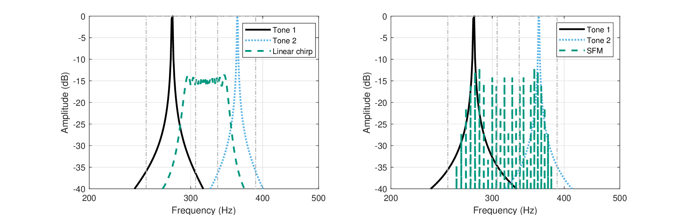
Figure 15.8: Examples for the combined spectra of two tones and a linear frequency modulated chirp with slope \(\Delta \dot{f} = 60\) Hz/s (left) or a sinusoidal frequency modulated (SFM) tone with \(f_m = 5\) Hz, \(\Delta f = 44\) Hz (right). In both cases, when played together, the FM sounds severely distorted, which may suggest a strong off-frequency phase distortion—a high-order aberration. The equivalent rectangular bandwidths of the filters centered at the tones are marked with dash-dot lines.

Several audio examples¹⁵³ are provided of clear cases where FM signals and tones are distorted. It is the impression of the author that for a relative level that is just about lower than the tones, most FM signals are severely distorted in the presence of the tones with high-frequency carriers, whereas at low frequencies the distortion to linear FM is more obvious than sinusoidal FM. In general, at low frequencies, the auditory filters are relatively broad (in terms of their bandwidth to center-frequency ratio), but occupy a small absolute frequency range, whereas at high frequencies they are relatively narrow, but occupy a larger frequency range in absolute terms. Thus, high-frequency channels encompass more phase cycles, which make phase aberrations there more likely. Several alternative explanations may be brought up, such as a masking effect by difference tones, strong instantaneous interference between the FM and the pure tone sounds, or a complex suppression pattern between the tones and the FM. As can be gathered from §15.4, these explanations are not necessarily in contradiction to the aberration one proposed here. It will be left for future experiments to determine—and for the reader to judge—which of the explanations is the most plausible.

At present, we shall retain the hypothesis that off-frequency higher-order aberration causes the loss of FM details. This is likely exacerbated by a mismatch between the phase aberration in the overlapping flanks of the two adjacent filters. The overall effect is blurring of the FM of the signal. It is possible that in typical acoustic objects and normal listening such extreme off-frequency responses are largely avoided due to the narrow bandwidth of the filters combined with lateral inhibition. Implications for the perception of temporal fine-structure in hearing-impaired listeners are discussed in §17.6.3.

15.10 Chromatic aberration

Polychromatic images may be subject to chromatic aberration that can give rise to a distinct type of blur. In spatial imaging, it occurs as a consequence of dispersion (also called in this context chromatic dispersion)—the dependence of the speed of light on wavelength in the optical medium. There are two main types of chromatic aberration. In axial or longitudinal chromatic aberration the focal length depends on the wavelength, so the different monochromatic images do not align in the same plane and are therefore not all equally sharp. In transverse or lateral chromatic aberration, magnification itself is wavelength dependent, so that off-axis images in different wavelengths do not exactly overlap (Charman, 1995; pp. 24.17–24.19; Miller and Roorda, 2010; pp. 15.22–15.23). Because of the relatively large bandwidth of visible light, axial chromatic aberration in the normal eye causes a shift in focus of 2.25 diopters between the short and long wavelength range of light (Packer and Williams, 2003; p. 58), whereas lateral chromatic aberration is 36 arcsec (Charman, 1995; p. 24.18) or \(\pm3\) arcmin (Miller and Roorda, 2010; p. 15.23), depending on how it is measured. While the ocular chromatic aberration probably does not have a perceptible blurring effect in normal vision (Packer and Williams, 2003; pp. 59–60), axial chromatic aberration must be compensated for in the design of virtually all polychromatic optical instruments.

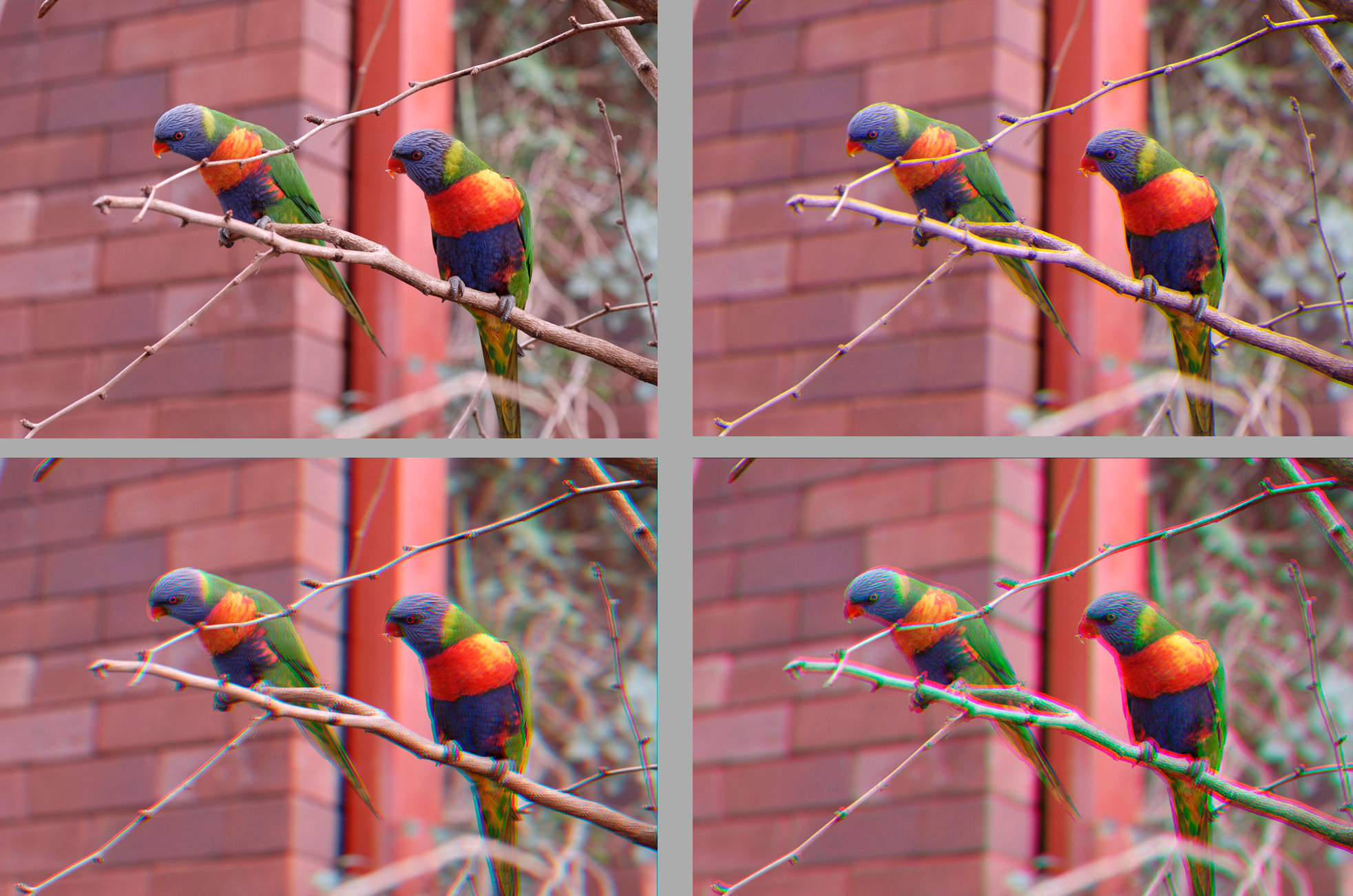
Figure 15.9: Blur caused by chromatic aberration. The polychromatic image on the top left is obtained by exactly aligning the three color channels (shown in Figure 15.5). By translating the monochromatic images by a few pixels relatively to each other, a gradually increasing blur may be observed, where the top right is slight blur (green 1 pixel to the right, 4 pixels up; red 2 right, 4 up), the bottom left medium blur (green 1 up, 4 left; red 1 up, 9 left) and bottom right most blur (green 6 left, 2 down; red 1 right, 4 up). Note how the effect of blur is strongest for the objects that are already in focus, whereas the effect on the out-of-focus background is much subtler. This figure is a spatial analogy to the temporal chromatic aberration. However, its blurring effect also resembles transverse chromatic aberration, which produces a distinct colorful halo around objects in the image. For example, on the bottom right photo, the twig on which the birds are sitting has a pink halo from above.

In temporal imaging, the dispersive effect causes envelopes that are carried by different frequency bands to be delayed in a frequency-dependent way. Thus, in broadband signals that are subjected to frequency-dependent dispersion, the envelope contents of different components do not arrive together. The corresponding form of chromatic aberration may therefore take place when the image of the polychromatic complex envelope is not temporally synchronized across channels. We shall refer to it as temporal chromatic aberration (cf. this term in ultrashort pulse optics, Andreev et al., 2008, and in motion vision, Mullen et al., 2003). An analogous visual effect is illustrated in Figure 15.9, where gradually increasing amounts of blur are produced by translating the monochromatic images (from Figure 15.5) by a few pixels, relatively to each other.

In most optical systems that employ ultrashort-pulse temporal imaging, it is unusual to have an ultra-wideband spectrum as is common in hearing (see §6.6.2), so chromatic aberration has not been formally analyzed. In spatial imaging, the dispersive and diffractive effects operate on different dimensions, so there are more degrees of freedom than in temporal imaging, also with regards to aberrations. In temporal imaging, frequency-dependent dispersion is the cause of group-delay dispersion, so some level of chromatic aberration is almost inescapable. Particularly, the very existence of defocus is indicative of its temporal chromatic aberration. This is because only a sharply focused system has a total group-velocity dispersion that is zero, which entails constant group delay. In contrast, the defocused system has a non-zero group-delay dispersion, which entails a non-constant group delay (Eq. §11.1). Because of the inherent defocus in the system, the role of axial chromatic aberration is not expected to be critical insofar as the individual channels are not sharply focused¹⁵⁴. However, the two other types of chromatic aberration will be explored below. Chromatic aberration will be a necessary building block in the analysis of hypothetical dispersive hearing impairments, where more results from literature will be analyzed (§17).

15.10.1 “Transverse” chromatic aberration

Up until this point, auditory magnification has not been given any explicit significance. However, its numerical proximity to unity may make its effect elusive. While the variation in magnification in most of the audio spectrum is not large—it varies by about 14% or less over three decades according to our estimates (reproduced in Figure 15.10, right), it can be expected to influence across-channel timing. This is because the local time variable is scaled by the channel magnification (even for a stationary pure tone) according to \(\tau \rightarrow \tau/M\), as dictated by both the focused and defocused imaging transforms of Eqs. §12.19 and §12.27, respectively. If pitch detection is a temporal process or is anyway conveyed by a local time variable, then even slight changes in magnification may lead to a discrepancy between the perceived pitch and the physical frequency prediction, which is scaled as the reciprocal of the time, \(f \rightarrow Mf\) (see also Bennett and Kolner, 2001, Eq. 27). This discrepancy enables us to tap into the effects of transverse chromatic aberration.

The magnification variation in frequency may be applicable in the analysis of the stretched octave phenomenon. In order to obtain a subjective octave perception of double the pitch of a two-note sequence¹⁵⁵, it is necessary to stretch the octave tuning to a slightly larger ratio than 2:1 (Ward, 1954). More specifically, the stretching effect levels off at 200–400 Hz of the reference tone (i.e., the lower note) and is stronger at high frequencies, but seems to be reduced with complex tones (Jaatinen et al., 2019). These relations are summarized in the left plot of Figure 15.10, which reproduces pure-tone data compiled from literature by Jaatinen et al. (2019, Figure 1), as well as from simulated musical instrument octaves across the musical range from the same article. Stretched intervals are so ingrained in musicians' hearing that Jaatinen et al. (2019) advocated for adapting the stretched tuning curve as a new standard that can replace the usual equal-tempered tuning¹⁵⁶.

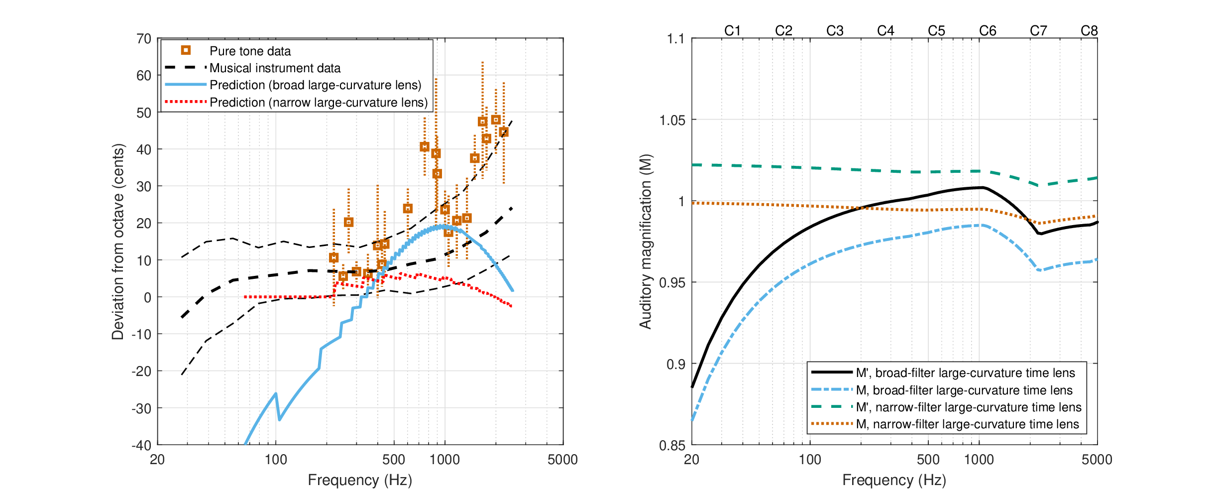
Figure 15.10: Magnification and stretched octave data. Left: Stretched octave psychoacoustic data and prediction reproduced from Jaatinen et al. (2019, Figure 1). The red squares and confidence intervals represent pure tone data compiled from literature by Jaatinen et al. (2019). The thick black dashed line is the threshold to their simulated orchestral instrument (complex tone) sounds, including its confidence intervals in thin dash black. The prediction according to auditory magnification is plotted twice, once for the broad-filter (large-curvature) time lens (solid blue) and another for the narrow-filter in dotted red, both according to Eq. 15.4. Right: The auditory magnification curve replotted from §11.6, for both filter types in the large-curvature time lens. Musical notes are marked on the top abscissa between C1 and C8 for reference.

Several hypotheses have been proposed that account for the stretched octave effect. They include an excitation pattern place model that is centrally learned just like speech (e.g., Terhardt, 1974), an auditory-nerve neural firing temporal model attributed to a frequency-dependent refractory period (Ohgushi, 1983; McKinney and Delgutte, 1999), and a cochlear model based on the geometry of outer hair cell row arrangement (Bell, 2019). A study by Hartmann (1993) of binaural Huggins pitch revealed the same octave stretched response as in diotic pure-tone tests, which led him to propose a modified neural timing model, based on autocorrelation. However, this model could not be corroborated using cat data (McKinney and Delgutte, 1999). This, as well as findings by Bonnard et al. (2013) and Demany and Semal (1990), disfavor the learned-template place model of Terhardt (1974), but do not explicitly rule out a central autocorrelation model. Additionally, McKinney and Delgutte (1999) reexamined Ohgushi's model and emphasized that the timing deviations that were attributed to refraction by Ohgushi (1978) may stem from an earlier (cochlear) cause.

A stretched octave theory should be also able to explain the difference between the pure tone and the complex tone values. It may be similar in nature to the difference between the melodic and harmonic octaves: as multiple partials vibrate together, there is a clear subjective tendency to prefer the “simple” over the stretched frequency ratio (Bonnard et al., 2013). This may represent a trade-off between the two pitch dimensions—tone chroma that is relevant for harmonic relations and tone height that is relevant to pure tones across the audible spectrum (Bachem, 1950; Warren et al., 2003).

A prediction based on the magnification ratio between the reference frequency and its octave, which are functions of local time variables, can be easily generated by looking at an auditory \(f_1\):\(f_2\) magnified interval, such that the two frequencies \(f_2 \approx 2 f_1\), which satisfies the relation:

\[ 2f_1 M(f_1) = f_2M(f_2) \]

(15.2)

where the magnification \(M(f)\) explicitly depends on frequency. This equation assumes that the locally perceived (magnified) frequencies have to be mathematically doubled in value in their internal auditory representation, in order for the interval to be perceived as having a true octave relation. Ideally, the magnification is exactly unity and \(f_2 = 2f_1\). In reality, there is a discrepancy, because \(M(f_1) \neq M(2f_1)\), so a different frequency \(f_2>2f_1\) has to be found to satisfy Eq. 15.2. For convenience, we can define the deviation between the ideal and the real frequency using \(\Delta f = f_2 - 2f_1\). Typically, the results in the cited studies are expressed in cents¹⁵⁷. Therefore, we take the logarithm base 2 of Eq. 15.2, multiply by 1200, and after some rearranging obtain

\[ 1200\left(\log_2 \frac{f_1}{f_2} + 1 \right) = 1200 \log_2 \frac{M(f_2)}{M(f_1)} \]

(15.3)

Using \(\Delta f\), we can obtain an expression that depends only on \(f_1\), albeit indirectly through \(M\)

\[ 1200 \log_2 \frac{M(f_1)}{M(2f_1 + \Delta f)} = 1200\left[\log_2 \left( \frac{\Delta f}{f_1} + 2 \right) -1 \right] \]

(15.4)

A graphical solution may be found by solving both sides of the equation for different \(\Delta f\) around \(2f_1\). Note that only when the magnification is identical at the two frequencies, then \(\Delta f = 0\). Note also that the magnification used may be either the general expression \(M = (v+s)/s\) (Eq. §12.16) or the effective magnification for the defocused pulse \(M'\) (Eq. §12.25), which also depends on the aperture size \(t_0\) and cochlear group delay dispersion \(u\), but produces the same predictions.

Ward (1954) and Jaatinen et al. (2019) emphasized and verified the requirement of interval additivity, which entails that the sum of the tuning factors for two consecutive intervals \(f_1\):\(f_2\) and \(f_2\):\(f_3\) must be equal to \(f_1\):\(f_3\). Using the magnification rule above, this requirement is automatically satisfied by virtue of having the frequency scaled by a multiplicative factor. If the first two magnified intervals are set according to

\[ I_1 = \frac{M_2f_2}{M_1f_1} \,\,\,\,\, I_2 = \frac{M_3f_3}{M_2f_2} \]

(15.5)

then their combined interval is

\[ I_3 = \frac{M_3f_3}{M_1f_1} = \frac{M_3f_3}{\frac{M_2f_2}{I_1}} = I_1 I_2 \]

(15.6)

which is a sum in the log cent scale, as interval additivity requires.

To the extent that the prediction correctly captures the stretch effect, it is limited in frequency to 200–500 Hz for the narrow-filter large-curvature time lens (red dotted curve, Figure 15.10, left), where the predicted effect is at most 5 cents. At higher frequencies, this curves remains flat and then decreases, opposite to empirical data where the stretch shoots up above 500 Hz. Similarly, the broad-filter large-curvature time lens roughly captures this stretch size increase at 500–1000 Hz, but completely misses the target outside this range. As the predicted octave stretching effect depends on the magnification \(M\), it is effectively dependent on the time-lens curvature \(s\) and on the neural dispersion \(v\) (but not on the cochlear dispersion \(u\)). The uncertainty we have in the estimates of \(s\), which has hitherto been of negligible importance, becomes particularly noticeable in modeling this phenomenon, as two different predictions in Figure 15.10 show. Note that at frequencies lower than 220 Hz, no empirical data is available (for pure tones), and the magnification values are also likely to be off, being based on untested assumptions and extrapolations (§11.6.3). The source of discrepancy above 1000 Hz is less certain and may be the result of mis-estimated \(s\), \(v\), or both. The other time lens estimates (the constant focal-time and small-curvature) all produced predictions that are completely off target and are not displayed here.

The temporal imaging theory considers the dispersive function of elements that are both peripheral and central, and requires both place and temporal theories to interact, in similarity to modern pitch theories (e.g., de Cheveigné, 2005; Moore, 2013; Oxenham, 2022). Place information determines the rough identity of the narrowband channel, whereas temporal information conveys the dynamics of the modulation variables. The magnitude of the magnification itself is dependent on the time lens and neural group-delay dispersion, but is negligibly dependent on the cochlear group-delay dispersion. Inasmuch as the magnification implicates the perception of pitch height, then both peripheral and central modeling have some merit, as the effect of the fine details of the dispersive elements may be factored into their group dispersive properties (e.g., a frequency-dependent neural refractory period). As temporal imaging is a coarse-grained approach to the auditory system, it is agnostic to the fine-grained explanations of the stretched octave that were mentioned above.

The smaller stretch factor required in complex tones may be explained using mode locking, rather than with dispersion. Mode locking causes an inharmonic overtone series to synchronize into a harmonic series. If a similar mechanism occurs in the auditory brain, then it may contribute to a significantly smaller stretch factor in complex tones. (See §9.7.2 for discussion¹⁵⁸).

Incidentally, the connection between pitch height and magnification may indirectly support the existence of a time lens in the system—something that was questioned in §12.7.5, given the similarity of the system to a pinhole camera design. This is important because the effect of the lens appears to be almost negligible in most other contexts (e.g., curvature and modulation perception), while it dominates magnification and keeps it at near unity level (Fig. §12.2). The magnification analysis may be a useful tool for calculating the individual human time lens properties indirectly, once the individual neural group-delay dispersion is known. For example, the stretched octave effect and data are used in §F along with three additional psychoacoustic effects to derive a strictly psychoacoustic estimation of all the dispersion parameters in the auditory temporal imaging system. That calculation was designed to perfectly match the empirical data. It produces a magnification that is much closer to 1 below 1000 Hz (\(M>0.966\)), which decreases more rapidly above. However, no estimate is available below 125 Hz.

The magnification analysis in conjunction with pitch perception lends itself to another interesting hypothesis, which is more general and is likely relevant even if the precise values of the magnification are still uncertain and do not produce satisfactory predictions. As is seen in Figure 15.10, at least one magnification estimated (based on the broad-filter curvature) is relatively flat in a narrow frequency range (200-1000 Hz), but it decreases more sharply in the bass and treble ranges. Comparing the frequency range in which the magnification is flat and close to unity with the melodic range in music (roughly C2–C6, where C4 is Middle C is set at 261.6 Hz), begs the question of whether the melodic range itself exists in the region of the flattest magnification. This range roughly contains the vast majority of melodic and harmonic instruments and spans the conventional ranges of bass, tenor, alto, and most of the soprano voice types.

Other side-effects of the auditory transverse chromatic aberration may exist that are not necessarily related to pitch, but depend on the magnification distortion of the local time variable.

A challenge that can be leveled against the magnified frequency explanation to the stretched octave effect is that it is not reflected in physiological measurements, which directly quantify the period in the auditory nerve and other pathways. These responses are locked to the input over the (usually long) time frames in which the neural activity recording takes place. In order for the magnification stretch and the long-term frequency synchronization to coexist, it entails that any scaling takes place on the image (sample) level that should correspond to perceived pitch, and/or is limited to shorter time frames. However, there is no evidence at present to support these ideas and more research will be needed to uncover the exact relations between these levels of operation.

15.10.2 Temporal chromatic aberration

The effect of temporal chromatic aberration on pulses is illustrated in Figure 15.7, as a simplified analogy to the spatial example of Figure 15.9. The figure shows the components of a modulated harmonic polychromatic tone, whose intensity envelopes are carried in four channels. The synchronized (coherent) version where the tone overlaps in all frequencies is the sharpest polychromatic image, whereas the aberrated version shows a blurring effect. Temporal chromatic aberration is nearly synonymous with group-delay distortion, which is known from audio engineering and is considered undesirable (e.g., Blauert and Laws, 1978; Flanagan et al., 2005), and in some cases is directly redressed by dedicated corrective filters (e.g., for the mixing sweet spot in a control room) that boast improved stereo imaging. However, group-delay distortion is rarely discussed with respect to its blurring effect (but see Davidson et al., 1999; p. 6-27).

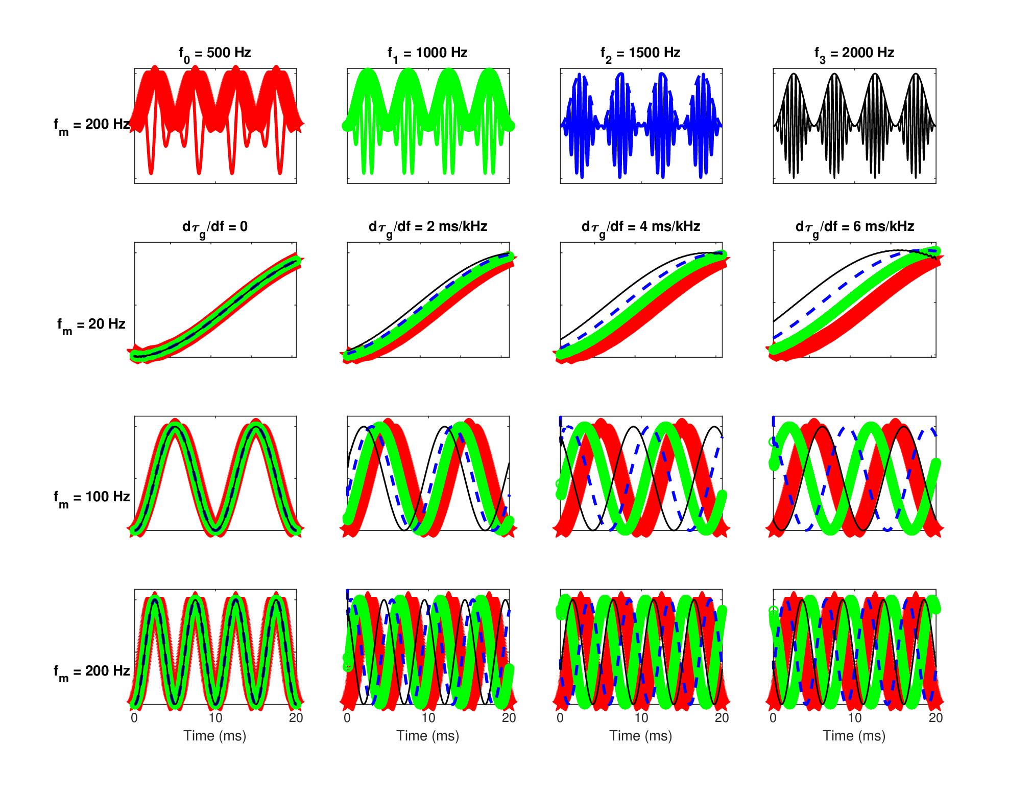
Figure 15.11: The effect of temporal chromatic aberration on an amplitude-modulated complex tone with \(f_0 = 500\) Hz and its first three harmonics. The four components (carriers and envelopes) are plotted separately in the top row of the figure, each with its own color and line-style to emphasize the analogy with spatial chromatic aberration. The image is the intensity envelope of the individual channels, indicated only with colors, but no carriers, which are assumed to have been removed after demodulation. When the group delay is identical in all channels (leftmost column), the polychromatic envelope shape is well-defined. As the group delay is increased (left to right), the blurring effect becomes more apparent, in an increasing manner with higher modulation frequencies (from top to bottom).

Just as in vision, it is necessary to distinguish between the intrinsic chromatic aberration of the auditory system, and the system's sensitivity to chromatic aberration induced by external factors. Evidence for the internal level of chromatic aberration may be gathered, for example, from click auditory brainstem response (ABR) dispersion, which is typically attributed to cochlear dispersion only, but actually accounts for the dispersion along the entire system. Don and Eggermont (1978) and Don et al. (1998), Don et al. (2005) isolated the contributions of different frequency bands to the broadband click ABR wave-V response and found 1–5 ms latency differences between high and low frequencies, depending on level and subject. Similar values may be gathered from the group delay measurements that were summarized in Figure §11.15 (left) based on several studies (Table §11.1), which were used for the derivation of the cochlear and neural group-delay dispersion.

The internal chromatic aberration pattern that exists in normal hearing under normal acoustic conditions may be assumed to be perceptually well-tolerated by design. This is supported by several psychoacoustic studies that show how clicks rather than chirps are perceived as the most compact stimuli (Uppenkamp et al., 2001), perhaps through central compensation of otherwise asynchronous channels (e.g., McGinley et al., 2012). A similar conclusion may be drawn from a study that found how the synchrony of two tones was perceived to be maximal when they were gated simultaneously, independently of the spectral distance between the two tones (Wojtczak et al., 2012). According to the pulse ribbon model, global (across-channel) phase misalignment is corrected centrally as long as the misalignment between channels is relatively small (4–5 ms across the bandwidth; Patterson, 1987 and §6.4.2). According to this model, only relatively large global phase effects could be heard.

The sensitivity to external chromatic aberration may be deduced in part from available psychoacoustic data. As was mentioned above, group-delay distortion threshold measurements essentially quantify the same function, but without an explicit reference to the temporal imaging quality and the effect on modulation. Relevant studies typically employed various all-pass filter designs, which were used to process the phase of broadband impulses, but only over a narrow spectral range (see review in Møller et al., 2007). The results varied depending on the specific methods, but showed group delay detection thresholds between 0.5 and 2 ms, with 1.5 ms being a typical average value that is relatively frequency-independent. The effect on the impulse sound was described as increased “pitchiness” or extended ringing. However, when applied to music or speech, the effect is often inaudible, probably due to masking (Møller et al., 2007). Nevertheless, an across-spectrum gradual delay was applied to speech in another line of studies, where tolerance in terms of intelligibility was assessed by delaying the large spectral ranges in a frequency-dependent manner. Performance is much more robust than may be inferred from the impulse response studies, as intelligibility dropped only with delays longer than 60 ms across the spectrum (Arai and Greenberg, 1998). High frequency bands, however, deteriorated more quickly with increasing delays with performance flooring at 240 ms. In another experiment where only two narrow bands of speech were presented, the performance was shown to depend much more critically on timing information and delays as short as 12.5 ms already had a strong effect (Healy and Bacon, 2007).

Audio examples that demonstrate the temporal chromatic aberration are provided in the audio demo directory /Section 15.10.2 - Chromatic aberration/, where a male speech excerpt was bandpass-filtered into seven bands, which were then summed back together, compensating only for the internal group delay of the center frequency of the filters. Other versions progressively applied differential group delay to the different bands before summing them up, in a way that sounds more and more objectionable, when the group delay is long enough. Very short group delays, however, are almost inaudible, in line with psychoacoustic studies. At relatively long group delays, the ringing effect (Møller et al., 2007) can be heard more as a “chirpiness”, because it is not confined to a single frequency. Intermediate group delays tend to sound more metallic. These group delays, however, do not seem sufficient to significantly degrade intelligibility of anechoic speech in quiet. It requires about 50–100 ms of delay between consecutive channels to render the speech unintelligible, albeit in a very artificial way.

15.11 Auditory depth of field?

The visual depth of field quantifies the distance range (from the lens) within which an object can be positioned in order to produce a sharp image (see examples in Figures §4.3 and 15.12). Blurred objects in a defocused spatial scene encroach into neighboring objects, as their contours and fine details blend in and the overall contrast in the corresponding area of the image is lost—depending on the amount of blur. For example, a close inspection of the tabletop texture in Figure 15.12 reveals how when the texture lines become blurry close to the lens they also become broader and fainter, until they completely disperse into a featureless surface. In contrast, in the focused area of the image, points of the object do not visibly encroach into the space of neighboring points, which remain well-resolved (by definition).

According to the space-time duality, if spatial depth of field manifests in space as a function of the spatial envelope that represents the object features, then the temporal depth of field should manifest temporally through changes to the temporal envelope. Similarly, the encroachment in space beyond the ideal-image locus due to spatial blur can be analogized to temporal features that encroach in time beyond the local time of their own coordinate system.

Figure 15.12: Depth of field as a function of focal length of the lens. In the photos, the sharp focus is set to be on the middle (green) cup or on the white cup in front of it. As the focal length is decreased (from left to right), the depth of field increases, which can be seen in the cups that are most distant from the lens, which are less blurry and in the background—the sky and the metal railing. Note how the visual attention is automatically drawn to the middle cups in the left photo, which are in sharp focus. This attentional effect is visible but weaker in the middle photo, but not so much in the right photo, which is perceived more as an aggregate and is also dominated by the magnified and blurry cups in the front. The region of sharpest focus and its surrounding blur can be clearly seen in the marks on the tabletop, which demonstrate how the depth of field increases for smaller focal length (on the right). The photos were taken with constant (nominal) f-number of f/2.8 and lenses of 85 mm, 50 mm, and 24mm focal length (from left to right, respectively). Additionally, in order to conserve the angular extent of the image, the camera was brought closer to the objects for smaller focal lengths, to obtain approximately the same image.

The spatial depth of field is determined by the focal length of the lens, the distance from the object to the lens, and by the relative aperture size—the f-number, \(f^{\#} = f/D\), where \(f\) is the focal length, and \(D\) is the aperture size (§4.2.1 and Eq. §4.5). Two parameters have an immediate counterpart in temporal imaging—focal time and f-number (see §15.11.1). A distance counterpart is more complicated, because it is the total amount of dispersion that we care about, irrespective of the distance over which it builds up. Also, the range of allowable group-delay dispersion is unintuitive and is not mapped well using the space-time analogy. Instead of a range of distances, we would ideally prefer to obtain a time interval. A simple manipulation of the imaging conditions can provide us with a suitable quantity (§15.11.2). Finally, we have to consider coherence as a parameter that is crucial in the auditory depth of field, but has no practical significance in vision (at least not in daily circumstances and natural light). We will consider this factor in §15.11.3. We will return to the question of focal time in §16.4.2.

15.11.1 The auditory f-number

An analogous temporal-imaging expression to the f-number that was proposed by Kolner (1994a) is simply

\[ f_T^{\#} = \frac{f_T}{T_a} \]

(15.7)

where \(f_T\) is the focal time and \(T_a\) is the aperture time. This number quantifies the inverse of the relative aperture time—how much of the signal energy enters the system for its particular configuration.

The auditory f-number according to Eq. 15.7 is plotted in Figure 15.13 for three lens curvature estimates we obtained in §11.6 and the aperture time from Table §12.2. In spatial imaging, the f-number represents the relative irradiance (intensity per unit area) that is available for the image and it should have a similar logic in hearing too. In the case of the auditory system, the combination with neural sampling and the fact that we have no reference for this number in other acoustic systems makes it somewhat difficult to interpret. More importantly, since the auditory system is defocused and it is governed by the signal coherence, the usefulness of the f-number concept is not exactly clear at this stage.

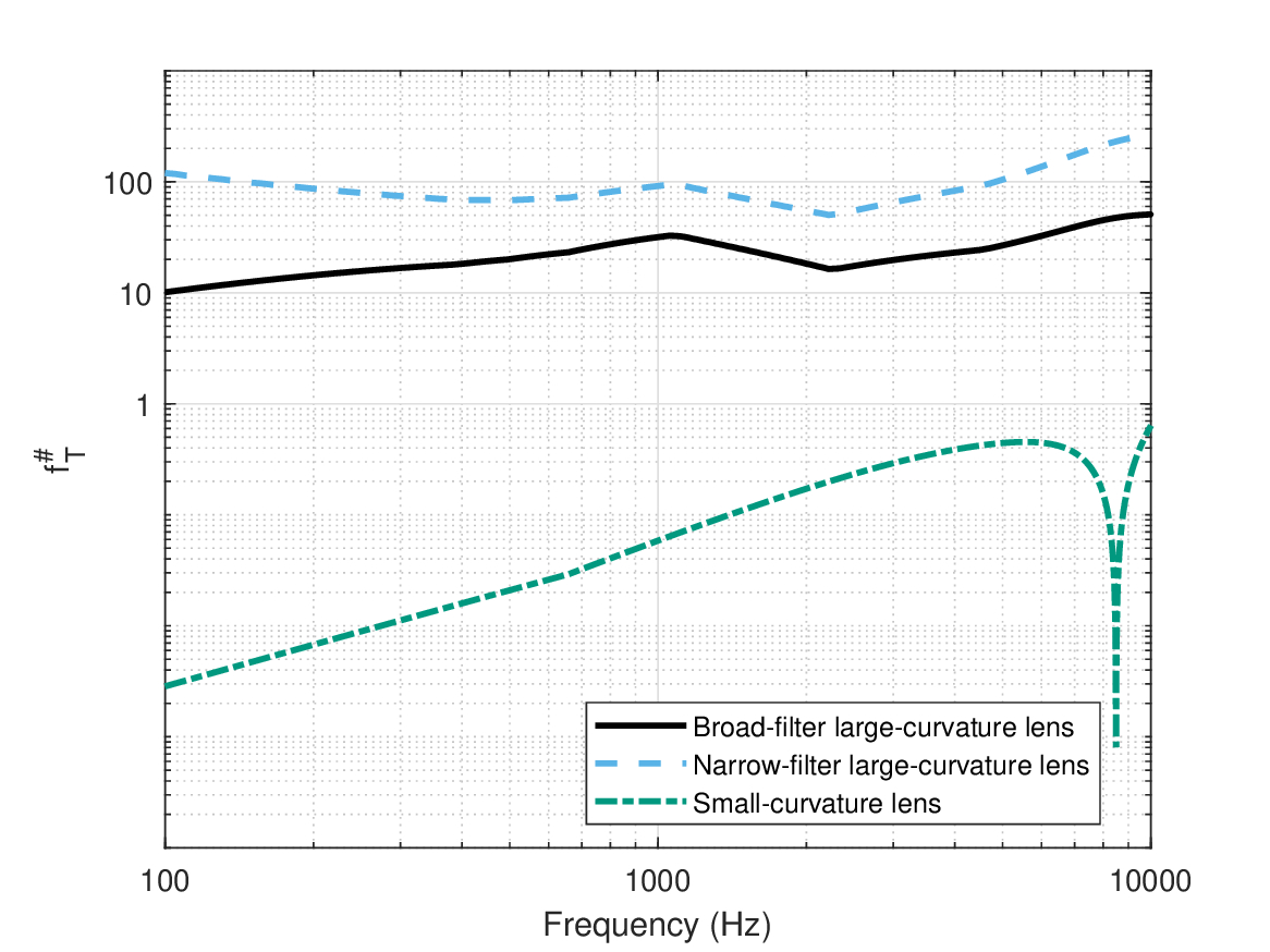
Figure 15.13: Estimated auditory f-number, based on three different time-lens curvatures: the broad-filter and the narrow-filter large-curvatures that have been used throughout the text, and the small-curvature time lens (the absolute value f-number displayed) that has been largely omitted from analyses due to its implausible values (§11.6).

15.11.2 Auditory depth of field (time)

The spatial depth of field is expressed as a range of distances for the imaging system, when it is in sharp focus. While we do not have a sharply focused system, we can use it as a starting point from which it may be possible to obtain a temporal quantity instead of group-delay dispersion. Starting from the imaging condition:

\[ \frac{1}{u} + \frac{1}{v} = -\frac{1}{s} \]

(15.8)

we can express \(s\) with the focal time (Eq. §10.32) and \(u\) and \(v\) with their group delay derivatives (Eq. §10.25) to get

\[ \frac{2}{\frac{d\tau_{g,u}}{d\omega}} + \frac{2}{\frac{d\tau_{g,v}}{d\omega}} = -\frac{2\omega_c }{f_T} \]

(15.9)

where \(\frac{d\tau_{g,u}}{d\omega} = 2u\) and \(\frac{d\tau_{g,v}}{d\omega} = 2v\). This expression entails

\[ \frac{1}{\omega_c \frac{d\tau_{g,u}}{d\omega}} + \frac{1}{\omega_c\frac{d\tau_{g,v}}{d\omega}} = -\frac{1}{f_T} \]

(15.10)

All terms of this expression have the dimensions of time and are determined by the center frequency of the time lens. As long as we stick to the narrowband approximation, this expression may be approximately correct also for off-frequency conditions. In the cochlea, however, we have assumed throughout the text (without proving) that time lensing is available on-frequency throughout the audible range. If this is so, then \(\omega_c\) can continuously vary with center frequency. Otherwise, it should be fixed to the channel carrier that is determined by the time lens. In analogy to spatial optics, in a sharply focused system that satisfies this condition, the depth of field should be defined for an interval of \(\omega_c \frac{d\tau_{g,u}}{d\omega}\) for which the image appears sharp. While this expression can endow us with the confidence that the depth of field can be expressed as a temporal range, it is not necessarily straightforward to apply in practice.

Empirical temporal ranges that can represent the depth of field may be derived from data of several psychoacoustics studies. To this end, we will reinterpret observations of asynchrony perception of different components of a polychromatic object that temporally stick out. Zera and Green (1993a) measured the effect of differentially gating the onset time of a single component of complex tone with a fundamental of \(f_0=200\) Hz and 20 components between 200 and 4000 Hz (Figure 15.14). Complex tones were defined by a “standard” asynchrony \(T\)—the delay time between the lowest and highest components of the tone, which could be either negative or positive. The other components were delayed accordingly, except for a single component, which started with an extra delay \(\Delta t\) that deviated from that standard. Subjects had to discriminate between the standard tone and the one that contained a delayed component. Measurements repeated for harmonic tones and logarithmically-spaced inharmonic tones in several conditions. In the harmonic condition, the in-phase components fused and formed an acoustic object whose highest harmonics were unresolved. In contrast, the inharmonic tone components were almost always resolved into separate auditory filters, but did not fuse to create unified perceptual objects. As the experiment manipulated the onset time of the components, it directly affected the (spectrotemporal) envelope, and hence the auditory image of the complex tones¹⁵⁹.

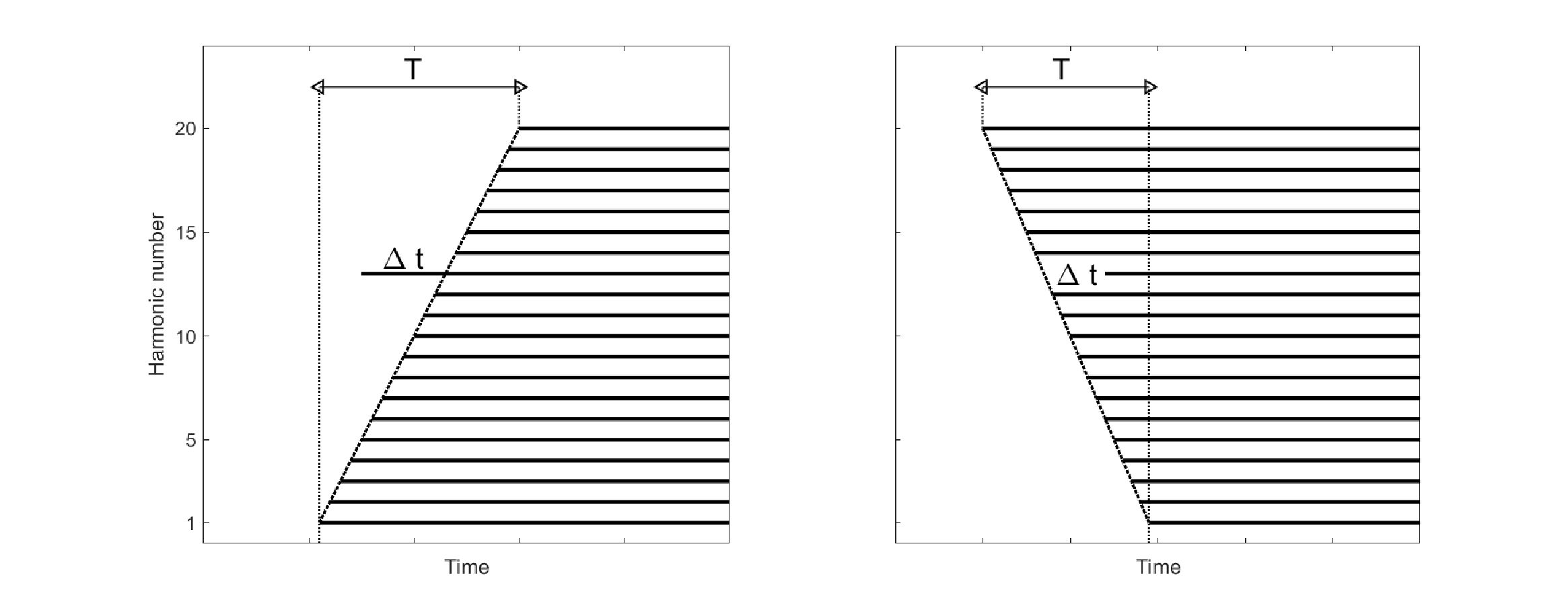
Figure 15.14: An illustration of the stimuli used in Zera and Green (1993a). Complex tones with 20 components were varied with respect to their relative onset time, whose asynchrony slope is determined by the standard \(T\), which may be either positive (left) or negative (right). An additional parameter is the deviation of a single component from the standard, \(\Delta t\), which can also be either positive or negative. Inharmonic versions of this stimuli were tested as well using the same number of components that were logarithmically spaced.

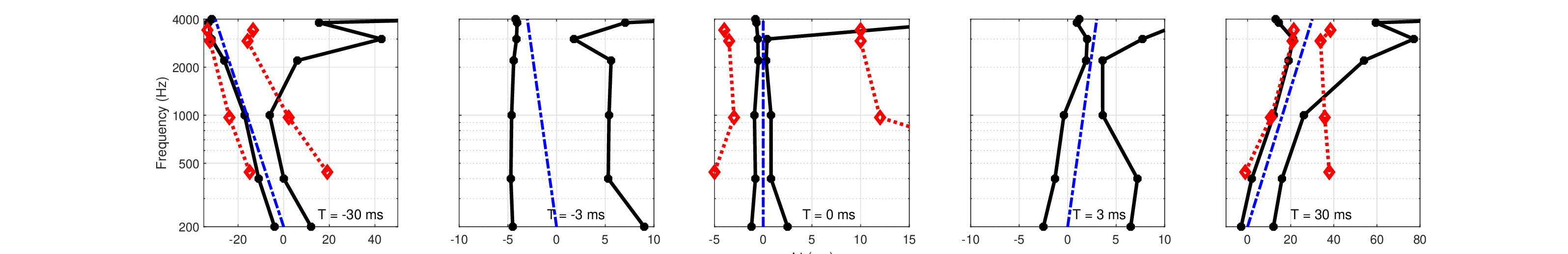
Figure 15.15: Replotted data from Zera and Green (1993a, Figures 2, 4, and 5), which show the discrimination threshold for a manipulated single component of harmonic and inharmonic complex tones, whose onset is delayed by \(\Delta t\) relatively to the tone onset standard, as shown in Figure 15.14. The complex tone standard is defined by the onset asynchrony of the components (\(T\)), which is defined as the delay between the lowest and the highest components. The standards are plotted with dash-dot blue lines and are, from left to right: -30, -3, 0, 3 and 30 ms. The negative values indicate that the high-frequency component onsets come first, whereas low-frequency component onsets come first when they are positive. Responses to harmonic tones (\(f_0=200\) Hz, 20 harmonics, zero initial phase for all components) are plotted in solid black and are based on three subjects, except for the \(\pm3\) ms conditions that are based on one subject. Inharmonic tones had the same fundamental frequency and number of components, but were logarithmically spaced at a 1.17 ratio between components. The responses to the \(T=\) -30, 0, and 30 ms inharmonic standards are plotted in dotted red and are based on two subjects. It is hypothesized here that the area bounded between the lines on both sides of the standard slope corresponds to the auditory depth of field of the ear for these stimuli.

The results of Zera and Green (1993a) are rearranged and replotted in Figure 15.15. There are at least two alternative ways to associate the depth of field with the results. Resolving the component from the complex tone is possible when both are sharp (large depth of field), or when one is sharp and the other is blurred (small depth of field). In general, the smaller the absolute value of the asynchrony is, the smaller is the effective depth of field, which is represented in the figure by the black contours for the harmonic tones and by red contours for the inharmonic tones. So, the highest sensitivity to single-component delays shows when all the tone components are in phase in the synchronous condition (\(T=0\), middle plot) with some specific components being as sensitive as \(\Delta t \le 0.6\) ms. Additionally, there is higher sensitivity to components starting before the standard than to those starting after (i.e., the solid black lines to the left of each standard in blue are closer to it than the solid black lines to its right). Importantly, the sensitivity to these early-onset components is relatively frequency-independent, with the synchronous condition varying by less than 1 ms throughout the entire spectrum (at least below 4000 Hz), in line with group-delay distortion detection studies (Møller et al., 2007). The exception are the two highest (unresolved) components tested of 3800 and 4000 Hz that produced anomalous thresholds of 40–100 ms in other conditions. The response to inharmonic tones (shown in red in three plots) is relatively frequency independent for \(T = \pm 30\) ms, but is more dispersed for \(T = 0\) ms and \(\Delta t < 0\). It should be noted that the synchronous results are similar to those obtained in Zera and Green (1993b, Figure 9), where it was found that increasing the number of delayed components in the harmonic condition further enhanced the sensitivity to changes (reduced \(\Delta t\)). The opposite occurred for the inharmonic tones (Zera and Green, 1993b; Figure 10). Discrimination thresholds also depended on the onset phase of the delayed component (Zera and Green, 1995).

These results from Zera et al. are telling about the system sensitivity to chromatic irregularities that affect its image. As they were tested specifically with complex tones, it is unknown to what extent they can be generalized. For example, does the in-phase standard \(T = 0\) elicit the minimum possible depth of field? Does it depend on the bandwidth of the complex tone? Is it highest for completely coherent stimuli? Also, these observations comprised data from three subjects or less, which is insufficient for more sweeping generalizations. Nevertheless, the data are in accord with related observations by Wojtczak et al. (2012) of a better-controlled, yet simpler across-frequency asynchrony detection task¹⁶⁰

15.11.3 Auditory depth of field (coherence)

The depth of field is generally defined with respect to an object in focus and is given as a range in dimensions of length. If we draw direct analogy between spectral and temporal imaging, then the analogous depth of field in temporal imaging systems should specifically relate to the sensitivity of the image to dispersive path from the object to the lens (Shateri et al., 2020)—a quantity that can be combined with the cochlear dispersion \(u\). As was discussed in §3.4, the farther the object is, the more dispersed it tends to be, subject to conditions in the environment. However, a much more dominant effect of the environment that interacts with dispersion is a general loss of signal coherence between the source and the receiver due to weather conditions, reflections, and noise—both coherent and incoherent. These effects also strongly depend on the acoustic source coherence, which dictates the kind of transformations that the waves may be most sensitive to (§8.2.5). Here, dispersion is only one factor that leads to signal decoherence, according to the signal bandwidth. Therefore, dispersion alone is probably not the most informative parameter that should be employed to characterize the auditory depth of field. But, if dispersion is considered along with source randomness, its effect can be approximated to decoherence, for a certain degree of detail or temporal resolution (see §82).

Given its similarity to the pinhole camera, we may expect the auditory system to have a relatively high depth of field for signals that are anyway in focus—namely, completely coherent narrowband stimuli, which are largely insensitive to defocusing, but are instead sensitive to interference and decoherence. In contrast, incoherent stimuli are sensitive to defocus, but not to interference and decoherence. Hence, partially coherent objects are sensitive to dispersion, interference, and decoherence in different amounts. This suggests a departure from the straight analogy to the spatial depth of field, as external coherence constitutes the most dynamic parameter of the environment and objects can vary in more than a single dimension (i.e., distance). Additionally, we should consider that the extensive signal processing in the auditory brain may be set to exaggerate the depth of field, as may be expected from a standard imaging system that is completely passive. Let us explore how the effective auditory depth of field may arise in common situations.

According to the space-time duality applied to the auditory depth of field, defocused temporal objects extend in time beyond the temporal boundaries of the original signal (from the acoustic source), which manifests somehow on the time-frequency plane¹⁶¹. If this is the case, then it should be possible to measure the effect of this extension, as the boundaries of the image encroach into the images of adjacent objects—both in time and in frequency. In other words, a finite auditory depth of field anticipates the existence of nonsimultaneous masking—the change in the response of one sound by another non-overlapping sound.

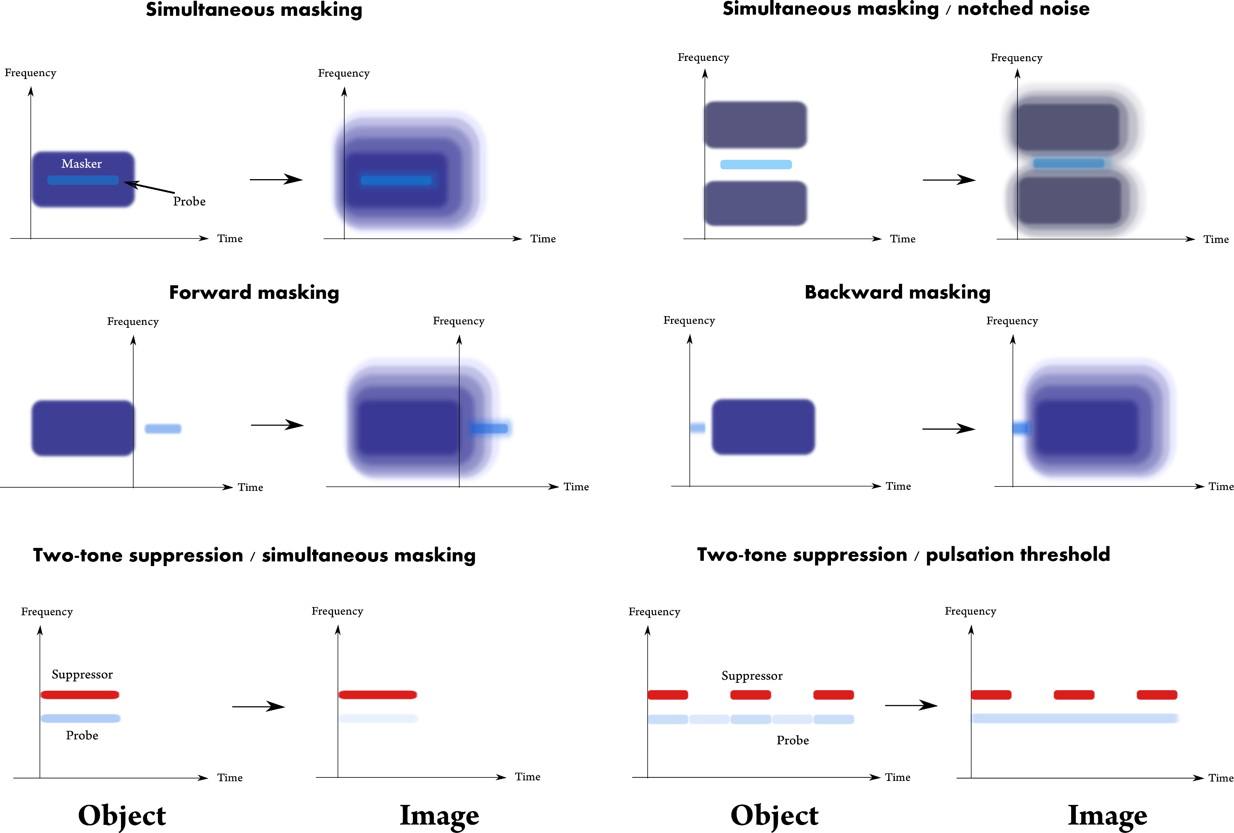
Figure 15.16: Cartoon summary of common types of masking paradigms reframed as objects and images on the time-frequency plane. The stimulus is considered the object and is illustrated on the left. It is perceived as an image, which is illustrated on the right of each pane. The rectangle designates the masker, which is usually a narrowband or broadband noise, although it is sometimes a sinusoid. The probe is typically a sinusoid whose frequency coincides with the center of the masker in on-frequency conditions. If it is presented with the masker, then it is referred to as simultaneous masking (top left). A variation on this type of masking is the notched-noise with tone, which has been extensively used to estimate the auditory filter bandwidth by varying the spectral gap between the two bands of noise (top right). In the example, the probe is “on-frequency”, as it is centered right in the middle of the notch. Non-simultaneous masking may be either forward masking, in which the probe is presented after the masker has been switched off (middle left), or the much weaker and shorter backward masking, in which a short probe is presented before the masker (middle right). Upon imaging, the masker gets a “halo”, so it extends beyond its original temporal and spectral limits in a diminishing way. When the masker image collides with that of the probe, it makes it more difficult to hear, which elevates its detection threshold. In the text, we refer to this extended blur between two objects as their relative depth of field. Objects are easier to tell apart over the background when they are sharp and the background is blurry. The bottom two plots describe two different effects of two-tone suppression. On the bottom left is the increase in the threshold of a tone as a result of another tone that is either higher or lower in frequency. On the bottom right is the pulsation threshold, which is the effect of a tone that is modulated, which sounds continuous at low thresholds as a result of another suppressing tone. Note that in the top four masking types, the image of the masker always extends asymmetrically toward high frequencies, in what is called upward spread of masking.

Nonsimultaneous masking

Typically, the stimuli used in nonsimultaneous masking experiments are classified as either maskers or probes according to the specific experimental paradigm that is being used (Figure 15.16). When the probe follows the masker, it is called forward masking (or postmasking), and the effect tends to be robust and extend up to 100–200 ms from the offset of the masker. When the probe precedes the masker, it is called backward masking (or premasking), and there the effect tends to be less robust and it operates on considerably shorter time scales (0–10 ms from the probe onset to the masker onset). Extensive literature exists about masking in general and about forward masking specifically, where it has been typically found that the exact change to probe threshold depends on all the stimulus parameters: the masker and probe duration, the gap between them, their absolute and relative levels, their absolute and relative spectra, the possible addition of more masking components, or the addition of other conditions (e.g., contralateral stimulation). The topic of nonsimultaneous masking is too vast to comprehensively treat here, in part because it is tightly related to the issues of frequency selectivity, temporal integration, compression, and suppression. We only review a handful of results that are amenable to the logic of temporal imaging and coherence, albeit in a more empirical way. Reviews of masking effects can be found in Fastl and Zwicker (2007, pp. 61–110) and Moore (2013, pp. 67–132). Early literature was reviewed by Duifhuis (1973).

There are two reference thresholds against which forward masking can be tested. When the masker and probe overlap, simultaneous masking may take place, which can be largely (but definitely not always) accounted for using energetic measures when the two stimuli are analyzed within the same auditory channel. Then, the signal-to-noise ratio (SNR) of the input (i.e., the probe-to-masker ratio) can be employed as the main parameter that explains the degree of masking (e.g., Fletcher, 1940). On the other extreme is the response to the probe in the absence of any masking. Forward masking is then the time-dependent residual masking between the simultaneous masking threshold and the threshold in quiet.

A central point in research about forward masking has been to account for the long time constants that are associated with the decay of masking after the external stimulus has long been switched off. At low frequencies, forward masking depends on the frequency of the stimuli, which suggests that the cochlear filter ringing may have some effect. But two more general mechanisms have been proposed to account for forward masking: neural adaptation in the auditory nerve and persistence of the stimulus in the central pathways (Oxenham, 2001). Adaptation may have a masking-like effect due to a reduction in spiking rate in the auditory nerve following the onset of the masker and subsequent slow recovery (Smith, 1977; Harris and Dallos, 1979). However, the physiological effect characteristics are inconsistent with psychoacoustic data, which have to consider detectability of the probe that is based on both the response and its variance (Relkin and Turner, 1988). Furthermore, listeners with cochlear implants also experience forward masking, despite the fact that their auditory nerve is directly stimulated without emulating adaptation (Dent and Townshend, 1987; Shannon, 1990). Also, it was found that centrifugal efferents to ventral cochlear nucleus (VCN) units in the guinea pig can either facilitate or delay the recovery from forward masking, beyond the response that is measurable in the auditory nerve (Shore, 1998). It has led to the conclusion that forward masking is caused by persistence that has a central origin, which may be modeled through temporal integration after preprocessing that occurs in the cochlea (Oxenham, 2001; DiGiovanni et al., 2018). This explanation defers the mechanism to yet unidentified brain circuits, although correlates have been found in the ventral and dorsal cochlear nuclei (Frisina, 2001), the IC (Nelson et al., 2009), and the auditory cortex (e.g., Calford and Semple, 1995; Brosch and Schreiner, 1997; Wehr and Zador, 2005). The forward masking effect seems to be largely complete at the level of the IC, where it was suggested that the neural persistence is the result of adaptation or offset inhibition (Nelson et al., 2009; Middlebrooks and Bremen, 2013). An analogous forward masking effect has been also found in amplitude and frequency modulated tones (Wojtczak and Viemeister, 2005; Byrne et al., 2012; Füllgrabe et al., 2021), but this type of masking (at least the AM) does not appear to be reflected in subcortical processing (Wojtczak et al., 2011).

Arguably, the conclusions from current research suggest that the auditory system is actively geared to produce and even exaggerate forward masking, rather than try to minimize it, as may be naively surmised from standard signal processing considerations. Indeed, it has been suggested that forward masking may be useful in object formation, as part of early scene analysis (Fishman et al., 2001; Pressnitzer et al., 2008). More germane to the present work, it further suggests that forward masking cannot be fully captured by the time-invariant imaging transfer functions. However, if the exaggerated function relies on a time-invariant imaging effect that is too short to be useful on its own (perhaps, similar in duration to backward masking), then new intuition may be garnered from qualitative depth-of-field predictions and observations. Specifically, if forward masking can be indeed reframed as a depth-of-field effect, then it should be possible to relate the coherence of both signal and masker to their measured response patterns. The coherence-dependent differences may be noticeable both in the magnitude and in the duration of the masking effects of stimuli of different kinds.

Nonsimultaneous masking as depth of field

Throughout this section, we have treated the masker and the probe as two temporally distinct objects in the external environment, whose corresponding images may be difficult to resolve because of masking that is generated internally, within the auditory system (Figure 15.16). We know from vision, by way of analogy, that the auditory depth of field should endow the listener with a percept to distinguish between foreground and background, but not between background and background or foreground and foreground. But, what is foreground and what is background between two acoustic objects? Since coherent signals are theoretically always in focus in the defocused system, then the relative degree of coherence between the objects may be a natural cue to distinguish between foreground and background. Thus, we would like to find out whether coherence can be used as a cue for masking release between these two images, which may then be reinterpreted as an auditory depth-of-field effect.

Two examples are presented that illustrate the effect of coherence on the depth of field. The first example is a simplified model of data presented by Moore and Glasberg (1985), which demonstrate a release from forward masking effect when a reference masker was mixed with another type of masker. We would like to show how the relative amount—or rather, the rank order of the relative amount—of masking release can be predicted from the coherence function. The reference masker was a 400 ms narrowband noise with 100 Hz bandwidth centered at 1 kHz, at 60 dB SPL, that included 5 ms cosine squared onset and offset ramps. The probe was a 20 ms 1 kHz tone burst at 60 dB SPL that had 5 ms onset and offset ramps and a 10 ms steady-state middle. The probe was presented immediately after the masker, at 0 ms offset-onset delay time. The authors mixed the reference masker with 75 dB SPL tones of 1.15, 1.4, 2, and 4 kHz, as well as 1.4 kHz tones at 50 and 60 dB SPL, and low-pass filtered (4 kHz cutoff) white noise at three different levels¹⁶². All masker combinations resulted in some release from masking—sometimes very substantial—that was presented as individual data for three subjects. The authors argued that the release from masking is unlikely to be caused by suppression for the majority of the masker types. Instead, they suggested it is caused by perceptual cueing, whereby the additional masker components disambiguate the masker and the signal where they are too similar to tell apart. The cueing relates to a nonspecific change in quality such as a level change, or any other temporal or spectral distinction that signals to the listener that the probe is distinct from the masker (Terry and Moore, 1977; Weber and Moore, 1981).

Perceptual cueing is a lower-level explanation of the more abstract depth-of-field effects that separate different types of objects according to their degree of coherence, which we argue is the most salient auditory analog to distance in vision. The coherence functions of the probe and the various maskers are plotted in Figure 15.17, for bandpass filtered stimuli. It can be seen from plot A in Figure 15.17 that the choice of narrowband masker and short tone burst produces coherence functions that are very similar, which means that the masker and stimulus are partially coherent to a similar degree. The fact that both have the same center frequency as well results in significant mutual coherence (cross-correlation) for the short temporal aperture duration that was applied (2.26 ms for 1 kHz; see Table §12.2). Mixing the maskers with additional components always results in a further decrease of mutual coherence (plots B–D), which effectively segregates the various probe-masker pairs. Within each plot, the smaller the slopes and maxima of the obtained coherence functions are relative to the masker-probe coherence in plot A, the larger is the release from masking. This can be compared to the measurements by Moore and Glasberg (1985) (shown in the legends of Figure 15.17), which correspond to the same rank order of coherence curve within each plot. However, the global rank order of the different stimuli does not correspond exactly to the measured one, possibly due to contributions from off-frequency channels (e.g., Moore, 1981), which were not modeled here.

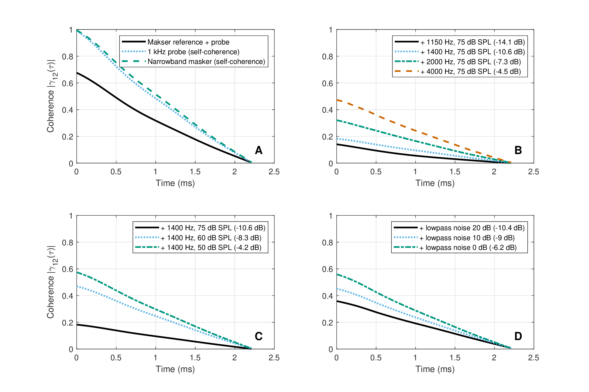
Figure 15.17: The coherence functions of the different maskers and probe from Moore and Glasberg (1985). The Hilbert envelope of the nonstationary coherence (Eq. §8.72) was obtained using the estimated aperture time at 1 kHz of 2.26 ms and 50% overlap between cross correlated segments (see §A.5). All stimuli are bandpass filtered at 1 kHz, using a second-order Butterworth filter. As the coherence function is symmetrical, it is displayed only for positive time. The results were averaged over 100 runs with randomized masker and noise. A: The self-coherence functions of the narrowband masker (centered at 1 kHz with 100 Hz bandwidth) and the probe (1 kHz tone), and their mutual coherence function. B–D: The mutual coherence of the narrowband masker and additional components with the tonal probe. The mean masking release compared to the reference masker is given in parentheses in the legend of all plots based on the three subjects in Table I of Moore and Glasberg (1985). B: Coherence of pure-tone maskers added to the reference. The closer the added component is to the 1 kHz probe, the lower is their degree of coherence, which results in higher release from masking. C: The same for 1.4 kHz tones at different levels. The higher the tone level is, the less coherent it is with the probe and the more release from masking is obtained. D: The same for low-pass filtered white noise at three different levels. The higher the noise level is, the lower is the coherence function which achieves increased release from masking.

The second example that illustrates the application of depth of field to forward masking presents the author's own data using all nine combinations of broadband, narrowband, and tonal maskers and probes. The three maskers were 100 ms in duration, where their onset and offset were ramped with cosine square functions over 5 ms. The narrowband masker was centered at 1000 Hz and was 100 Hz wide. The sine masker was a 1000 Hz tone and 10 ms with the same 5 ms ramps at onset and offset with no steady-state portion. The sine and narrowband maskers were normalized to have the same RMS level, but the broadband masker was set to 10 dB lower (RMS) to have approximately equal loudness for the three maskers, at a comfortable listening level. The forward masking thresholds for different offset-onset delay values are plotted in Figure 15.18 grouped for probes and maskers, referenced to the threshold at 400 ms delay. The simultaneous masking thresholds were measured as well, as an additional reference. The results follow the familiar forward masking patterns that were sometimes modeled as exponential decay (e.g., Plomp, 1964b) with much of the decay taking place within the first 10 ms and then more slowly up to 200 ms and beyond.

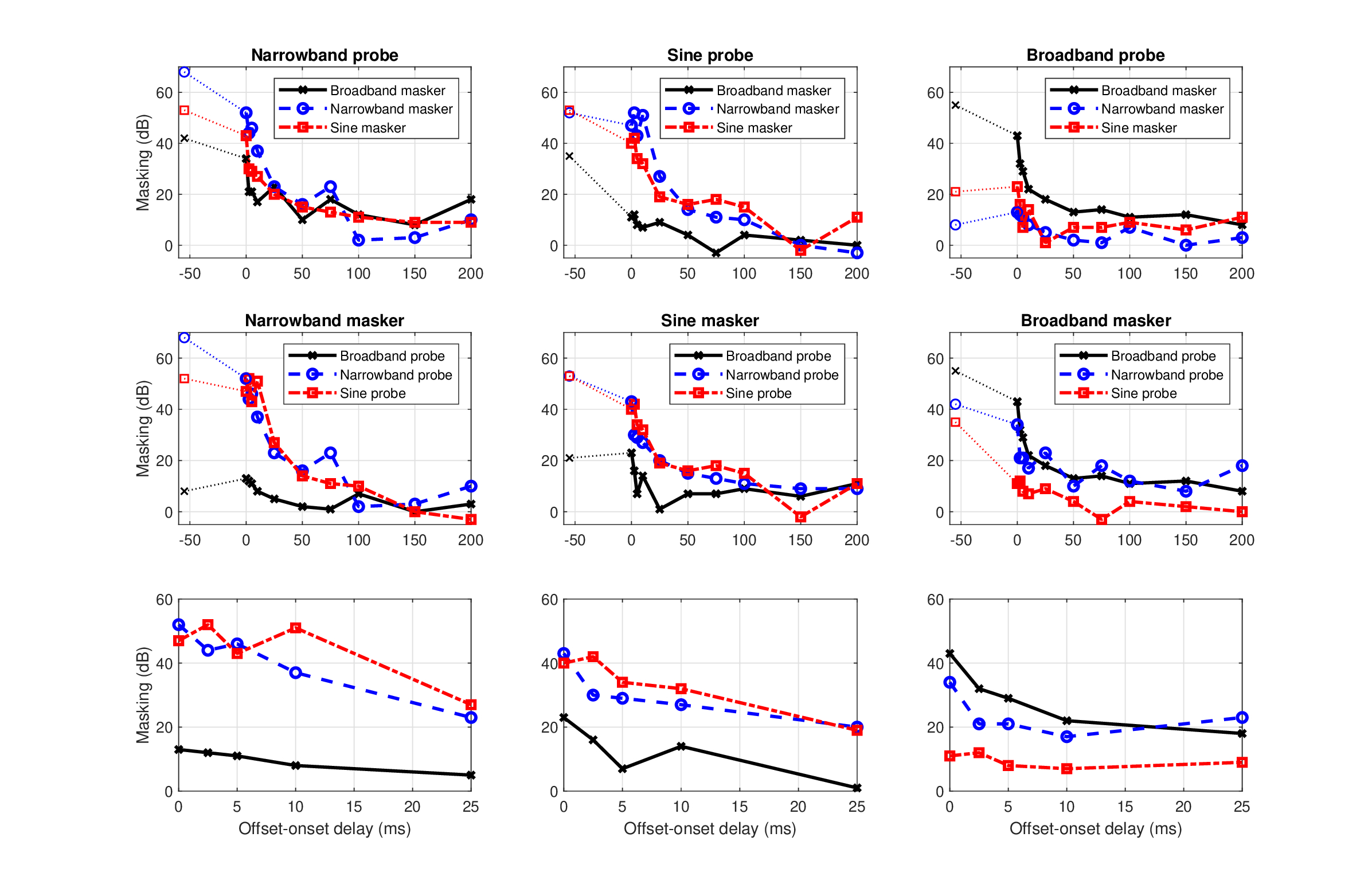
Figure 15.18: Forward masking decay curves for three masker and probe combinations of a single normal-hearing listener. The masker was always 100 ms and the probe 10 ms, both with 5 ms cosine squared fades. The sine masker and probe are at 1000 Hz, and the narrowband is centered at 1000 Hz with 100 Hz bandwidth. The broadband masker and probe were full bandwidth. Offset-onset delay times tested were 0, 2.5, 5, 10, 25, 50, 75, 100, 150, 200, and 400 ms. The amount of masking was referenced to the threshold measured with an onset-offset delay of 400 ms (not shown). Simultaneous masking thresholds were also measured for probes that were exactly centered within the maskers and are shown at -55 ms with dotted lines. The two top rows contain the same data organized according to common masker or common probe. The third row contains the same information as the second row, but zoomed in on offset-onset delays of 0–25 ms. The root mean square (RMS) level of the sine and narrowband maskers were equalized and the broadband masker was set to -10 dB from that value to be approximately the same loudness. The absolute presentation level could not be determined, but it was fixed at a comfortable level. The testing equipment was identical to that described in §F.1.4.

The most striking aspect in the results of Figure 15.18 is that the masker is always highly effective for a probe of the same type: broadband for broadband, narrowband for narrowband, and sine for sine. In contrast, masking is least effective for the most dissimilar types: narrowband and sine maskers for broadband probes, and broadband masker for sine probe. In the other cases, the sine and narrowband probes tend to behave similarly and elicit about the same thresholds in the case of narrowband and sine maskers, but somewhat more masking in the case of broadband masker and narrowband probe.

As before, these results are intuitively explained, in part, by appealing to coherence. Roughly speaking, the broadband stimuli are incoherent and the narrowband are partially coherent. The sine masker is close to being fully coherent, whereas the sine probe is also partially coherent due to its short duration—perhaps similar to the narrowband probe. This is captured in part in Figure 15.19, which again brings the mutual coherence curves of all masker-probe combinations. If we look at the rank order of forward masking at 0 ms, as in the first example, then most of the main trends are well predicted by the curves with the exception of the broadband masker and probe case. In this case the coherence calculation predicts to have the least masking of all pairs, which was not the case. Off-frequency modeling of coherence using additional channels can easily achieve the correct rank order of these pairs, but it has not been pursued here.

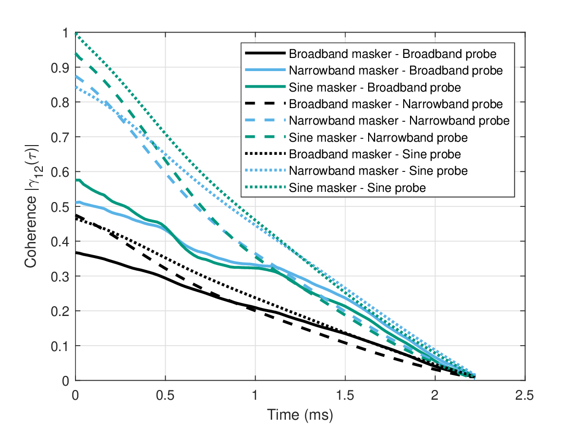
Figure 15.19: Mutual coherence plots of the stimuli described in Figure 15.18, computed as were detailed in Figure 15.17. Masker-probe pairs that are have higher mutual coherence are expected to be less easily distinguishable and hence elicit higher forward masking compared to those with low mutual coherence function. However, the predictions are not always correct here, as can be seen in the case of the broadband masker-probe pair. This may be explained by considering that the coherence modeling here was done on a single channel, whereas the broadband stimuli are multichannel.

Regardless of the modeling details, the main result stands: signals of different degrees of coherence elicit less masking the more dissimilar they are. This is measurable both in the threshold themselves, beginning in the simultaneous masking thresholds, and continues to the decay function, which determines the rate of release from masking. This was also seen in the comparisons between sine and narrowband masker-probe pairs in Weber and Moore (1981), where differences were attributed to both stimulus energy and perceptual cueing. These findings underline how the system is geared to differentially process objects according to their individual signal properties, such as their degree of coherence.

15.11.4 Discussion

The auditory depth of field is not entirely analogous to the visual depth of field, since there is no naturally-occurring coherence variation in optical objects that produce images whose sharpness is not affected by their distance from the eyes¹⁶³. Even pure tones, which we had considered to be in sharp focus in standard temporal imaging processing (§15.5), produce substantial forward masking when paired as both masker and probe, unless they are sufficiently well-separated in frequency (e.g., Miyazaki and Sasaki, 1984). In contrast, if a sharply-focused optical object is visually imaged, then an adjacent object at the same distance is not going to differ in relative sharpness as a result of a depth-of-field effect. The simple (and likely, simplistic) examples we explored revealed that objects may be differentiated according to their relative degree of coherence, but they do not exhibit preferential sharpness of a specific type of object as a function of its coherence. Therefore, the degree of coherence is not exactly analogous to distance in spatial optics and vision. This subtle point highlights the importance of partial coherence as the default mode of operation of the auditory system (see also §9.11, §16.4.8, §18.4.4, §18.4.5, and throughout §16).

Nevertheless, more realistic and complex stimuli may shed light on the idea of auditory depth of field. We explored rather narrowly the effect of coherence, but there are clearly additional parameters that determine the effective auditory depth of field such as dispersion, focal time, and f-number. Moreover, given that the auditory system clearly exaggerates the forward masking, it is not impossible that it can also control masking release under some conditions that are more dynamic in nature. We will touch upon this idea in §16 in the context of accommodation. Future studies will ultimately enable us to determine how useful this concept actually is within hearing science.

A final cartoon analogy of visual objects is displayed in Figure 15.20. It illustrates how different relations between shape parameters (brightness, size, shape, relative distance, and blur) can determine the relative visibility of a small and dim “probe” next to a large and bright “masker”. These images do not appear as real spatial depth-of-field effects of a real complex scene, but rather underscore how the complex interplay between all object parameters affects perception that gives rise to the sense of foreground and background among the images. This figure is a reminder of how all factors may matter in the scene analysis and not all of them are necessarily acoustic or peripheral, when it comes to auditory processing, since attention, context, and other high-level cognitive factors all provide input to perception.

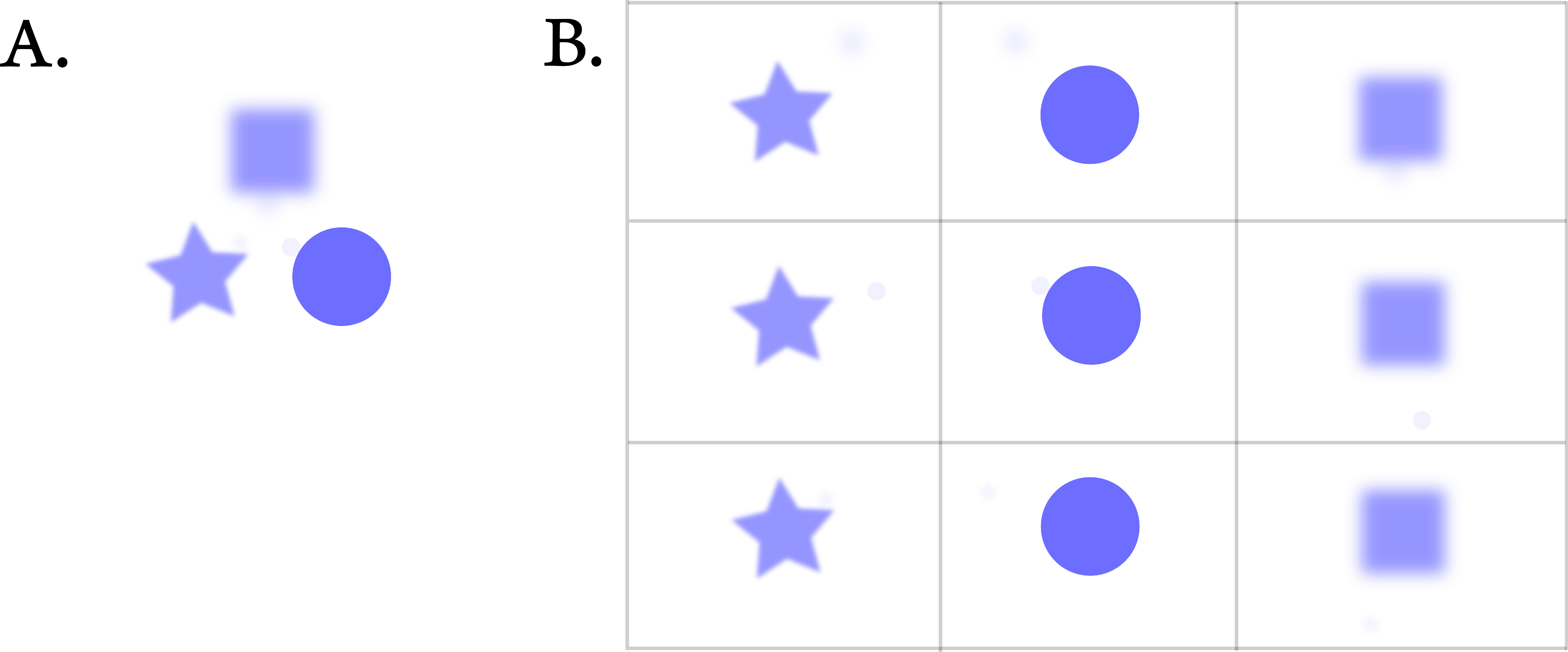
Figure 15.20: A visual analogy of auditory depth of field. Different shapes relate to different auditory objects. They vary in size, brightness, position, and blur, but not in color. A large and bright shape corresponds to a loud masker. A small dim shape corresponds to a probe. In A, all the maskers are displayed with the probes just next to them. In B, the nine probe-masker (small-large shape) pair combinations are displayed. Some probes are more readily detectable than others, based on their relative position to the masker and their degree of blur, which determines the sharpness of their contour. Note that this analogy does not map easily to the three masker and probe types used above (i.e., broadband, narrowband, sine). Still, it illustrates how all the parameters in the simple “scenes” are relevant to the detection.

15.12 Aberrations not found in hearing

Because of the lower-dimensional space of the temporal image compared to the spatial image, some of the most important aberrations in optics are irrelevant, as they require at least two spatial dimensions to manifest. Specifically, these are astigmatism, which causes blur because of asymmetrical focus about the optical axis that causes the loss of rotational symmetry, and curvature of field, which happens when the image is projected on a flat plane but is in fact focused on a curved surface (Born et al., 2003; pp. 240–244). It may be argued, though, that curvature of field is possible in temporal imaging as well, if the sharp image is formed on a mathematically curved surface in the time domain. However, such an effect in a single dimension may then be expressed as a combination of spherical aberration and distortion. In hearing, analogous aberrations to these two—if they exist—may manifest in nontrivial ways, such as in the binaural integration to a unitary image from the individual channels. These aspects may be more pertinent to bat echolocation fidelity, for example, or in applications where high-precision, spatially-faithful, three-dimensional audio reproduction is of primary interest.

15.13 Aberrations due to nonlinearities

Ideal temporal imaging, as does any type of imaging, requires linearity of its lens (Kolner, 1994a), so there is a design advantage in obtaining auditory components that are not dependent on the signal amplitude. However, the question of whether the human auditory curvature is amplitude-dependent has not been settled. There is psychoacoustic evidence for linearity (Summers, 2000; Oxenham and Dau, 2001a; Tabuchi et al., 2016) and against it (Shen and Lentz, 2009). Similarly, there is physiological data from animals that suggest that the instantaneous frequency is amplitude-dependent (Wagner et al., 2009), and amplitude-independent (Carney et al., 1999; de Boer and Nuttall, 1997; Recio et al., 1997), at least up to input levels of 80 dB SPL. Other more well-studied aspects of the auditory system are definitely nonlinear whenever the outer hair cells are involved. This includes the time-lens curvature phase modulation that appears to depend on level (§11.6.3), as well as amplitude dependence of the complete dispersive pathway in the auditory system that was seen in auditory brainstem response and otoacoustic emission measurements (§11.7.3). Whether, and if so how, any of these amplitude dependencies affect the final image quality is presently unknown and is beyond the scope of this work.

15.14 Rules of thumb for auditory imaging

Seven rules of thumb are given below that encapsulate some of the intuition about the nature of the auditory image. They are all corollaries of having a partially coherent intensity imaging system, which has the object coherence as its currency. The first three are more-or-less synonymous with one another and are readily supported through empirical findings from literature, so they merely rephrase known system behavior that describe different aspects of auditory interference. The fourth one is a general corollary of the previous rules and much of the acoustic source analysis in §3. The last three are more directly drawn from analogies with optics and vision.

Note that throughout this work, the term “image” is used in three different meanings. First, it refers to a single image of the pulse object—the sample. This is equivalent to a “sound pixel”. Second, it is the time sequence of samples within a channel, which corresponds to a monochromatic image. Finally, it is the combined sequences of all channels, which give rise to a polychromatic image. It also includes any cross-channel effects that have to do with harmonicity. We have mainly referred to the second image type, although explicit calculations were done using the first image type only.

1. Coherent and partially coherent signals interfere within the auditory filter—Within a duration that is determined by the aperture stop of a single channel, signals may interfere through the superposition of their complex amplitudes, according to their degree of coherence. This is the case in the simple beating effect (see §8.2.9 and §12.5). More complex interference patterns are heard with the addition of tonal components within the same channel. For example, the timbre produced by complex tones or vowels that contain high-frequency harmonics that are not resolved can exhibit sensitivity to phase (see review of related phenomena in Moore, 2002). Other narrowband sounds also interfere intermittently (§13.5) or cause suppression partly because of cochlear dispersion. which can also be taken as a form of interference (§15.3.3). Incoherent signals or signals that are resolved in separate channels do not interfere, by definition. The image of an individual channel is approximately monochromatic.
2. An intensity-image is perceived at the auditory retina and more centrally—Despite the interference effects throughout the early auditory stages, the final image is perceived as an intensity pattern. Therefore, there is no perceptual positive or negative amplitude, but rather a strictly scalar sensation of level. So, in the simple beating example, the modulation frequency heard in beating is double than is implied by the amplitudinal interference (\(\Delta f\) instead of \(\Delta f/2\))

   \[ I(t) \propto p^2(t) \propto \cos^2(\pi\Delta f t) = \frac{1 + 2\cos (2\pi\Delta f t)}{2} \]

   (15.11)

   This holds also for frequency-modulated sounds, which are represented as intensity images that are manifested in dynamic pitch.

3. Polychromatic (broadband) images may mask, but they do not interfere—The superposition of monochromatic images (i.e., in different carriers with overlapping modulation spectra) does not lead to destructive interference. However, images in different channels are not independent either, since the information across channels can be pooled in different ways if they are coherent in envelope (§15.7). In the case of simultaneous but dissimilar intensity envelopes in different channels, listening in the dips may be possible, as quiet instances of one envelope overlap high-level informative instances of the other, just enough to enable speech recognition (Miller and Licklider, 1950; Cooke, 2006; Edraki et al., 2022). In other conditions, dissimilar images may mask one another or compete for attention.
4. Real-world signals that are partially coherent produce mixed behavior—Unlike visual objects, acoustic objects of auditory significance are very often nearly coherent over behaviorally-meaningful durations (§8.3). However, this coherence tends to be lost over distance, with reflections, and with reverberation (§8.4). Therefore, the most general type of auditory stimulus is partially coherent. It means that the response to arbitrary sounds is somewhere between the coherent and incoherent modes—interference tends to be partial as well. The response to the superposition of a sound and its own reflection also obeys their relative coherence time¹⁶⁴.
5. Pitch is the closest percept in hearing to color in vision—While there are numerous examples of stimuli that produce either pitch or color in nontrivial ways, in their most mathematically straightforward elicitation (pure tones / primary colors), they both refer to carrier channels of sound or light. Therefore, these sensory channels may be treated as communication channels, irrespective of their modality. Each channel is itself monochromatic, but the availability of multiple channels, which are also ordered on a continuous scale (cyclical or not), makes color and pitch comparable. The specific combination of light wavelengths can give rise to the perception of secondary or nonbasic colors that are elicited by a simple mapping to the three primary colors. In sound, these chromatic combinations may reflect some aspects of timbre (including temporal variations of timbre that are analogous to spatial variations of color). The analogy clearly breaks down when harmonicity is included, at least as a spectral domain phenomenon. Human vision is effectively less than one octave wide (Table §1.2), so the very possibility of harmonic effects is excluded by its limited bandwidth. However, temporal pitch or periodicity pitch can be directly gathered from the envelope, so analogies to optical periodicity in the spatial envelope domain may have some merit.
6. The characteristic frequency of the auditory channel corresponds to the optical axis of the eye—An object point on the optical axis should suffer no aberrations and obtain an ideal image. In hearing, this limit can be achieved only by the pure tone. This represents the fundamental assumption we have made—the paratonal approximation, which is analogous to the paraxial approximation in optics. This assertion should be qualified, though, since the visual and the optical axes of the eye are not exactly aligned, and there is a blind spot on the retina, which does not have an auditory analog.
7. Depth of field is measured over time, between temporally close objects—The blurring effect is exaggerated by the auditory system in the form of forward masking. Objects that sound similar and share similar coherence properties tend to mask one another more effectively than objects that are acoustically dissimilar and do not correlate well with each other. This may aid the listener in the formation of perceptual objects that are distinct from a competing background.

15.15 Discussion

This chapter began with an open question about the possible meaning of sharp auditory images. Instead of answering it directly, it led to an extensive analysis of the possible sources of aberration and blur in the system—some of which are hypothetical at present. This knowledge allows us to answer what sharp images are like, mainly by understanding what they are not: they do not suffer from any significant blurring aberrations. Namely, sharp auditory images are minimally defocused, exhibit negligible temporal and transverse chromatic aberrations, and inasmuch as they exist, they do not suffer from spherical and coma aberrations. Several extrinsic factors were mentioned as well that can blur acoustic objects and make them fuzzy upon arrival to the ears: high reverberation and multiple reflections, large distances, and turbulent atmospheric conditions. However, the acoustic source itself may be unstable, if it intrinsically produces aperiodic sound that varies too quickly for the auditory system to settle, which elicits a fuzzy auditory sensation. By definition, these are incoherent sources, which have random attributes that dominate their sound generation.

The relationship between sharpness and defocus in the hearing system is less obvious than in vision, due to considerations of coherence and phase perception, which do not exist in vision. Sharp images are unlikely to be audibly defocused, which means that the corresponding objects should have a high degree of coherence. Specifically, images of narrowband objects (either as standalone components, or as polychromatic combinations of sharp components) may have a “well-behaved” phase-function that is insensitive to defocus. In parallel, avoidance of chromatic aberration implies high across-channel coherence, which is both spectral and temporal. But, as the system appears to generally detect signals both coherently and noncoherently, the ideally combined image may be partially coherent, in reality. This means that a combination of defocus and decoherence may come into play within the imaging system and contribute to the perceived image. These considerations also permeate the logic of auditory depth of field, which provides a handle on temporal distinction between acoustic objects of different degrees of coherence. Some of these ideas will be explored in the next chapter, where different accommodating mechanisms are hypothesized that all require different capabilities of dynamic changes in the system signal processing.

In practice, no spatial imaging system can be designed to be aberration-free and different types of aberrations may have to be traded off (Mahajan, 2011; Born et al., 2003; pp. 243–244). An equivalent statement has not been proven for temporal imaging, but if it is understood mathematically as a one-dimensional analog of spatial imaging, there is no reason to expect it to be any different. If the existence of aberrations in auditory images can be established, then it opens the door for a novel assessment of sound perception that is much more rigorous than is in use today, whether in normal audio perception, or in hearing impairments. In any case, much work will have to be done to establish baseline performance levels and methods to measure them before such a feat may be possible.

Another potential use for the auditory aberration concept may be the elimination of higher-order aberrations from normal hearing. In vision, it has been shown that visual acuity can be improved beyond its normal function by optically correcting for coma and spherical aberrations that characterize the normal eye (Liang and Williams, 1997; Yoon and Williams, 2002). While a similar target seems to be far from our current understanding of the auditory system, it is not unthinkable that similar manipulations may be possible there too. Hearing systems that have evolved to be exceptional in some animals like bats and dolphins may have evolved to have relatively aberration-free hearing that is closer to be dispersion-limited than in humans.

Aberrations will provide an important stepping stone with respect to the analysis of hearing impairments, which will be attempted in §17.

Footnotes

141. In fact, the amplitude transfer function squared, \(|ATF|^2\), was used in the coherent case.

142. Refer to the audio demos in the directory /Figure 15.2 - auditory defocus/ to listen to the corresponding stimuli.

143. Mathematically speaking, this procedure is not strictly valid, as stochastic signals do not have a proper time-domain representation. This is regularly circumvented in optics using measurable autocorrelation and intensity functions, as was discussed in §13.3. Because of the low-frequencies involved, obtaining an ad-hoc time-domain representations for white noise is technically straightforward in acoustics and hearing. However, a more mathematically rigorous procedure may have to be developed for partially coherent signals—something that should be relevant in hearing as well.

144. The gap detection predictions are not very sensitive to the time-lens curvature, if the large curvature values are used.

145. Kiang (1990) discussed whether all the fibers that synapse to a single inner hair cell have correlated responses. While no direct multi-unit data were available that could be confidently be associated with the same hair cell, he surmised that the correlation between fibers is partial, at best. Nevertheless, we maintain that whatever correlation exists between fibers, it must depend on the stimulus coherence at the point of transduction.

146. For a review of the above phenomena, see Hall et al. (1995). Related examples of multichannel images and speech segregation are discussed in Patterson et al. (1992), who had already recognized that CMR is an interesting test case in their Auditory Image Model. However, no interpretation was offered there as for the underlying cause of this effect.

147. Any phase difference or time delay between a pure tone and its replica only causes the degree of coherence to become complex, but its absolute magnitude does not change, \(|\gamma|=1\) (see §8.2.1).

148. Borrowing from the concept of degenerate frequencies in physics (e.g., Goldstein et al., 2014; pp. 464–466).

149. Julesz and Hirsh (1972) considered the possibility to have the horizontal spatial dimension in vision analogous to auditory time and the vertical spatial dimension analogous to frequency. If this were the case, then harmonic relations could be presented geometrically using shapes with integer ratios. However, this is an arbitrary analogy that bears little physical resemblance to the complexity that is offered by real harmonicity.

150. Shamma (2001) argued that periodicity pitch perception is analogous to bilateral symmetry in vision, as both provide grouping and segregation mechanisms that can be used in the perception. This analogy relies on coincidence detectors that perform the comparison between inputs to different spectral/spatial channels. However, it is not clear why this analogy should be more appropriate than directly comparing the (bilateral) spatial dimensions of both senses, as hearing can detect spatial symmetry as well. Additionally, this analogy does not address the special status that integer ratios between multiple channels have in hearing, but not in vision that is only trichromatic.

151. It can be argued that over-modulation and off-frequency excitation are essentially the same thing, only that over-modulation is typically symmetrical around the carrier (characteristic frequency), whereas off-frequency is generally asymmetrical.

152. Rays that cross the optical axis at the position of the aperture stop (chief rays) are aberration-free by definition. In analogy, the center frequency of the temporal channel is aberration-free.

153. The examples are found in audio demo directory /Figure 15.20 - Higher-order aberration/.

154. Interestingly, a beneficial role in cephalopods (octopus, cuttlefish, and squid) of inherent axial chromatic aberration has been hypothesized and demonstrated in simulation, where the amount of blur along the optical axis can provide sensitivity to color in an otherwise monochromatic-photoreceptor visual system (Stubbs and Stubbs, 2016).

155. The two-tone sequence refers to a melodic octave, as opposed to a simultaneous harmonic octave, which is generally perceived more closely to the physical 2:1 ratio (Demany and Semal, 1990; Bonnard et al., 2013).

156. The effect is considered to be a likely cause for the standard practice in piano tuning to have octaves stretched, although another potential cause may be an attempt to reduce unwanted beating from the inharmonic partials of the piano (Railsback, 1938; Fletcher and Rossing, 1998; pp. 388–390).

157. One octave is logarithmically divided into 1200 cents, so a semitone is 100 cents.

158. Note that we distinguished this type of mode locking from other harmonic synchronization effects that were measured in the auditory brainstem and were also referred to as mode locking in the hearing literature.

159. Responses for offset gating were tested as well, but are not treated here. They were usually worse (less sensitive) than onset responses.

160. Using the common jargon in hearing research, when the depth of field is applied to polychromatic images, then they are considered “coherent”, as their temporal modulation is in phase. It is commonly used to describe stimuli rather than images. Combining the two terminologies, the depth of field relates to the set of objects that sound the same and may be considered effectively coherent for the subject. It should be stressed, though, as was argued in §7, this terminology is ambiguous, because it relates to different things in the carrier and modulation domains.

161. Forward masking in the temporal domain does exist in vision, where the perceived object size that is followed by a flash of light changes over 300 ms after the object disappears (Wilding, 1982). A much smaller effect exists if the object is preceded by the flash (backward masking condition). The effect is monoptic and may be a result of retinal processes only. Arguably, this type of masking does not satisfy the space-time analogy, as was defined earlier.

162. An additional contralateral condition was not modeled and is omitted here. However, a recent model by Encke and Dietz (2021), Encke and Dietz (2022) quantitatively accounts for the release from masking in a broad range of binaural conditions using interaural coherence, at a higher level of precision than was obtained (or attempted) here. The complex-valued coherence was derived from the spectral coherence (cross-spectral density function) using gammatone filter transfer functions to model the auditory filters and signal detection theory to model the subjective threshold.

163. We did see an example in §15.5 for an artificial visual system that exploits coherence to maintain sharp text for any focal length that the lens assumes (von Waldkirch et al., 2004).

164. Some of these effects are treated as part of the (monaural) precedence effect by distinguishing between signals that are fused (usually within an early 1–5 ms window), or perceived as separate for longer intervals (that become distinct echoes if very long). In the binaural effect, a distinction is also made for a shift in localization that characterizes signals with very short delays (\(<1\) ms) (Litovsky et al., 1999; Brown et al., 2015). In our framework, it would be natural to expect three regimes that correspond to fusion (coherence) and echo (incoherence), but also including a long intermediate one of coloration (§3.4.4), which corresponds to partial coherence between signals. In binaural hearing, which has received most of the attention in this line of research, there is an additional dimension of spatial coherence that is not directly relevant in monaural or diotic hearing.

References

Andreev, Sergei A, Greenfield, Dmitriy E, Monastyrskiy, Mikhail A, and Tarasov, Victor A. Spatial and temporal focusing of femtosecond electron bunches in time-dependent electric fields. Physics Procedia, 1 (1): 273–283, 2008.

Arai, Takayuki and Greenberg, Steven. Speech intelligibility in the presence of cross-channel spectral asynchrony. In Proceedings of the 1998 IEEE International Conference on Acoustics, Speech and Signal Processing, ICASSP'98, volume 2, pages 933–936. IEEE, 1998.

Arthur, RM, Pfeiffer, RR, and Suga, N. Properties of `two-tone inhibition' in primary auditory neurones. The Journal of Physiology, 212 (3): 593–609, 1971.

Bachem, Albert. Tone height and tone chroma as two different pitch qualities. Acta Psychologica, 1950.

Bech, Søren and Zacharov, Nick. Perceptual Audio Evaluation: Theory, Method and Application. John Wiley & Sons, Ltd., Chichester, England, 2006.

Bell, Andrew. A natural theory of music based on micromechanical resonances between cochlear sensing cells. Journal of Hearing Science, 9 (3), 2019.

Bennett, Corey V and Kolner, Brian H. Aberrations in temporal imaging. IEEE Journal of Quantum Electronics, 37 (1): 20–32, 2001.

von Bismarck, Gottfried. Sharpness as an attribute of the timbre of steady sounds. Acta Acustica united with Acustica, 30 (3): 159–172, 1974.

Blackledge, J. M. Quantitative Coherent Imaging: Theory, Methods and Some Applications. Academic Press, London, England, 1989.

Blauert, J and Laws, P. Group delay distortions in electroacoustical systems. The Journal of the Acoustical Society of America, 63 (5): 1478–1483, 1978.

Bonnard, Damien, Micheyl, Christophe, Semal, Catherine, Dauman, René, and Demany, Laurent. Auditory discrimination of frequency ratios: The octave singularity. Journal of Experimental Psychology: Human Perception and Performance, 39 (3): 788, 2013.

Born, Max, Wolf, Emil, Bhatia, A. B., Clemmow, P. C., Gabor, D., Stokes, A. R., Taylor, A. M., Wayman, P. A., and Wilcock, W. L. Principles of Optics. Cambridge University Press, 7th (expanded) edition, 2003.

Bregman, Albert S. Auditory Scene Analysis: The Perceptual Organization of Sound. MIT press, 1990.

Brosch, Michael and Schreiner, Christoph E. Time course of forward masking tuning curves in cat primary auditory cortex. Journal of Neurophysiology, 77 (2): 923–943, 1997.

Brown, Andrew D, Stecker, G Christopher, and Tollin, Daniel J. The precedence effect in sound localization. Journal of the Association for Research in Otolaryngology, 16 (1): 1–28, 2015.

Buus, Søren. Discrimination of envelope frequency. The Journal of the Acoustical Society of America, 74 (6): 1709–1715, 1983.

Byrne, Andrew J, Wojtczak, Magdalena, and Viemeister, Neal F. Forward masking of frequency modulation. The Journal of the Acoustical Society of America, 132 (5): 3375–3386, 2012.

Calford, Mike B and Semple, Malcolm N. Monaural inhibition in cat auditory cortex. Journal of Neurophysiology, 73 (5): 1876–1891, 1995.

Carney, Laurel H, McDuffy, Megean J, and Shekhter, Ilya. Frequency glides in the impulse responses of auditory-nerve fibers. The Journal of the Acoustical Society of America, 105 (4): 2384–2391, 1999.

Carney, Laurel H. Supra-threshold hearing and fluctuation profiles: Implications for sensorineural and hidden hearing loss. Journal of the Association for Research in Otolaryngology, pages 1–22, 2018.

Charaziak, Karolina K, Dong, Wei, Altoè, Alessandro, and Shera, Christopher A. Asymmetry and microstructure of temporal-suppression patterns in basilar-membrane responses to clicks: Relation to tonal suppression and traveling-wave dispersion. Journal of the Association for Research in Otolaryngology, 21 (2): 151, 2020.

Charman, Neil. Optics of the eye. In Bass, Michael, Van Stryland, Eric W., Williams, David R., and Wolfe, William L., editors, Handbook of Optics. Fundamentals, Techniques, & Design, volume 1, pages 24.3–24.54. McGraw-Hill Companies Inc., 2nd edition, 1995.

de Cheveigné, Alain. Pitch perception models. In Plack, Christopher J, Oxenham, Andrew J, Fay, Richard R., and Popper, Arthur N., editors, Pitch. Springer, 2005.

Chi, Taishih, Gao, Yujie, Guyton, Matthew C, Ru, Powen, and Shamma, Shihab. Spectro-temporal modulation transfer functions and speech intelligibility. The Journal of the Acoustical Society of America, 106 (5): 2719–2732, 1999.

Christiansen, Simon Krogholt and Oxenham, Andrew J. Assessing the effects of temporal coherence on auditory stream formation through comodulation masking release. The Journal of the Acoustical Society of America, 135 (6): 3520–3529, 2014.

Cohen, Marion F and Chen, Xiaofen. Dynamic frequency change among stimulus components: Effects of coherence on detectability. The Journal of the Acoustical Society of America, 92 (2): 766–772, 1992.

Cooke, Martin. A glimpsing model of speech perception in noise. The Journal of the Acoustical Society of America, 119 (3): 1562–1573, 2006.

Crouzet, Olivier and Ainsworth, William A. On the various influences of envelope information on the perception of speech in adverse conditions: An analysis of between-channel envelope correlation. In Workshop on Consistent and Reliable Acoustic Cues for Sound Analysis, Aalborg, Denmark, 2001.

Dabelsteen, Torben, Larsen, Ole Næsbye, and Pedersen, Simon Boel. Habitat-induced degradation of sound signals: Quantifying the effects of communication sounds and bird location on blur ratio, excess attenuation, and signal-to-noise ratio in blackbird song. The Journal of the Acoustical Society of America, 93 (4): 2206–2220, 1993.

Dau, Torsten, Kollmeier, Birger, and Kohlrausch, Armin. Modeling auditory processing of amplitude modulation. I. Detection and masking with narrow-band carriers. The Journal of the Acoustical Society of America, 102 (5): 2892–2905, 1997a.

Dau, Torsten, Kollmeier, Birger, and Kohlrausch, Armin. Modeling auditory processing of amplitude modulation. II. Spectral and temporal integration. The Journal of the Acoustical Society of America, 102 (5): 2906–2919, 1997b.

Demany, Laurent and Semal, Catherine. Harmonic and melodic octave templates. The Journal of the Acoustical Society of America, 88 (5): 2126–2135, 1990.

Dent, LJ and Townshend, BS. Backward and forward masking for direct electrical stimulation of the VIIIth nerve in two profoundly deaf subjects. The Journal of the Acoustical Society of America, 82 (S1): S72–S72, 1987.

DiGiovanni, Jeffrey J, Lynch, Erin E, Nagaraj, Naveen K, and Ries, Dennis T. Dominance of persistence over adaptation in forward masking. Attention, Perception, & Psychophysics, 80 (7): 1863–1869, 2018.

Doleschal, Florian and Verhey, Jesko L. Comodulation masking release with random variations of flanking-band center frequencies. The Journal of the Acoustical Society of America, 148 (2): 692–700, 2020.

Dolležal, Lena-Vanessa, Tolnai, Sandra, Beutelmann, Rainer, and Klump, Georg M. Release from informational masking by auditory stream segregation: Perception and its neural correlate. European Journal of Neuroscience, 51 (5): 1242–1253, 2020.

Don, Manuel and Eggermont, JJ. Analysis of the click-evoked brainstem potentials in man using high-pass noise masking. The journal of the acoustical society of America, 63 (4): 1084–1092, 1978.

Don, Manuel, Ponton, Curtis W, Eggermont, Jos J, and Kwong, Betty. The effects of sensory hearing loss on cochlear filter times estimated from auditory brainstem response latencies. The Journal of the Acoustical Society of America, 104 (4): 2280–2289, 1998.

Don, Manuel, Kwong, Betty, and Tanaka, Chiemi. A diagnostic test for ménière's disease and cochlear hydrops: Impaired high-pass noise masking of auditory brainstem responses. Otology & Neurotology, 26 (4): 711–722, 2005.

Drullman, Rob, Festen, Joost M, and Plomp, Reinier. Effect of temporal envelope smearing on speech reception. The Journal of the Acoustical Society of America, 95 (2): 1053–1064, 1994a.

Drullman, Rob, Festen, Joost M, and Plomp, Reinier. Effect of reducing slow temporal modulations on speech reception. The Journal of the Acoustical Society of America, 95 (5): 2670–2680, 1994b.

Duifhuis, H. Consequences of peripheral frequency selectivity for nonsimultaneous masking. The Journal of the Acoustical Society of America, 54 (6): 1471–1488, 1973.

Eddins, David A, Hall III, Joseph W, and Grose, John H. The detection of temporal gaps as a function of frequency region and absolute noise bandwidth. The Journal of the Acoustical Society of America, 91 (2): 1069–1077, 1992.

Edraki, Amin, Chan, Wai-Yip, Jensen, Jesper, and Fogerty, Daniel. Spectro-temporal modulation glimpsing for speech intelligibility prediction. Hearing Research, 426: 108620, 2022.

Elhilali, Mounya, Ma, Ling, Micheyl, Christophe, Oxenham, Andrew J, and Shamma, Shihab A. Temporal coherence in the perceptual organization and cortical representation of auditory scenes. Neuron, 61 (2): 317–329, 2009.

Encke, Jörg and Dietz, Mathias. The complex-valued correlation coefficient accounts for binaural detection. arXiv preprint arXiv:2111.04637, 2021.

Encke, Jörg and Dietz, Mathias. A hemispheric two-channel code accounts for binaural unmasking in humans. Communications Biology, 5 (1): 1122, 2022.

Ewert, Stephan D and Dau, Torsten. Characterizing frequency selectivity for envelope fluctuations. The Journal of the Acoustical Society of America, 108 (3): 1181–1196, 2000.

Fastl, Hugo and Zwicker, Eberhard. Psychoacoustics: Facts and Models. Springer Science & Business Media, 3rd edition, 2007.

Fishman, Yonatan I, Reser, David H, Arezzo, Joseph C, and Steinschneider, Mitchell. Neural correlates of auditory stream segregation in primary auditory cortex of the awake monkey. Hearing Research, 151 (1-2): 167–187, 2001.

Flanagan, Sheila, Moore, Brian CJ, and Stone, Michael A. Discrimination of group delay in clicklike signals presented via headphones and loudspeakers. Journal of the Audio Engineering Society, 53 (7/8): 593–611, 2005.

Fletcher, Harvey. Auditory patterns. Reviews of Modern Physics, 12 (1): 47–65, 1940.

Fletcher, Neville H and Rossing, Thomas D. The physics of musical instruments. Springer Science+Business Media New York, 2nd edition, 1998.

Fontaine, Bertrand, Köppl, Christine, and Peña, Jose L. Reverse correlation analysis of auditory-nerve fiber responses to broadband noise in a bird, the barn owl. Journal of the Association for Research in Otolaryngology, 16 (1): 101–119, 2015.

Formby, C. Differential sensitivity to tonal frequency and to the rate of amplitude modulation of broadband noise by normally hearing listeners. The Journal of the Acoustical Society of America, 78 (1): 70–77, 1985.

Forte, Antonio Elia, Etard, Octave, and Reichenbach, Tobias. The human auditory brainstem response to running speech reveals a subcortical mechanism for selective attention. eLife, 6: e27203, 2017.

Frisina, Robert D. Subcortical neural coding mechanisms for auditory temporal processing. Hearing Research, 158 (1-2): 1–27, 2001.

Füllgrabe, Christian, Sek, Aleksander, and Moore, Brian CJ. Frequency selectivity in the modulation domain estimated using forward masking: Effects of masker modulation depth and masker-signal delay. Hearing Research, 405: 108244, 2021.

Glasberg, Brian R and Moore, Brian CJ. Derivation of auditory filter shapes from notched-noise data. Hearing Research, 47 (1-2): 103–138, 1990.

Gockel, Hedwig E, Carlyon, Robert P, Mehta, Anahita, and Plack, Christopher J. The frequency following response (FFR) may reflect pitch-bearing information but is not a direct representation of pitch. Journal of the Association for Research in Otolaryngology, 12 (6): 767–782, 2011.

Goldstein, Herbert, Poole Jr., Charles P., and Safko, John L. Classical Mechanics. Pearson Education Limited, Harlow, UK, 3rd edition, 2014.

Goodman, Joseph W. Introduction to Fourier Optics. W. H. Freeman and Company, New York, NY, 4th edition, 2017.

Green, David M. Temporal acuity as a function of frequency. The Journal of the Acoustical Society of America, 54 (2): 373–379, 1973.

Haggard, MP, Hall III, JW, and Grose, JH. Comodulation masking release as a function of bandwidth and test frequency. The Journal of the Acoustical Society of America, 88 (1): 113–118, 1990.

Hall, Joseph W, Haggard, Mark P, and Fernandes, Mariano A. Detection in noise by spectro-temporal pattern analysis. The Journal of the Acoustical Society of America, 76 (1): 50–56, 1984.

Hall, JW, Grose, John H, and Mendoza, Lee. Across-channel processes in masking. In Moore, Brian CJ, editor, Hearing. Handbook of Perception and Cognition, pages 243–266. Academic Press, Inc., London, United Kingdom, 2nd edition, 1995.

Hanna, Thomas E. Discrimination and identification of modulation rate using a noise carrier. The Journal of the Acoustical Society of America, 91 (4): 2122–2128, 1992.

Harris, David M and Dallos, Peter. Forward masking of auditory nerve fiber responses. Journal of Neurophysiology, 42 (4): 1083–1107, 1979.

Hartmann, William Morris. On the origin of the enlarged melodic octave. The Journal of the Acoustical Society of America, 93 (6): 3400–3409, 1993.

Healy, Eric W and Bacon, Sid P. Effect of spectral frequency range and separation on the perception of asynchronous speech. The Journal of the Acoustical Society of America, 121 (3): 1691–1700, 2007.

van der Heijden, Marcel and Joris, Philip X. Cochlear phase and amplitude retrieved from the auditory nerve at arbitrary frequencies. Journal of Neuroscience, 23 (27): 9194–9198, 2003.

Helmholtz, von Hermann. Handbuch der physiologischen Optik. Verlag von Leopold Voss, Hamburg und Leipzig, 3rd ed. edition, 1909.

Houtgast, Tammo. Psychophysical evidence for lateral inhibition in hearing. The Journal of the Acoustical Society of America, 51 (6B): 1885–1894, 1972.

Houtgast, Tammo and Steeneken, Herman JM. A review of the mtf concept in room acoustics and its use for estimating speech intelligibility in auditoria. The Journal of the Acoustical Society of America, 77 (3): 1069–1077, 1985.

Huss, Martina and Moore, Brian CJ. Dead regions and noisiness of pure tones. International Journal of Audiology, 44 (10): 599–611, 2005a.

Huss, Martina and Moore, Brian CJ. Dead regions and pitch perception. The Journal of the Acoustical Society of America, 117 (6): 3841–3852, 2005b.

Jaatinen, Jussi, Pätynen, Jukka, and Alho, Kimmo. Octave stretching phenomenon with complex tones of orchestral instruments. The Journal of the Acoustical Society of America, 146 (5): 3203–3214, 2019.

Julesz, Bela and Hirsh, Ira J. Visual and auditory perception: An essay of comparison. In David, EE and Denes, P, editors, Human Communication: A Unified View, pages 283–340. McGraw-Hill, New York, 1972.

Katz, Jack, Chasin, Marshall, English, Kristina, Hood, Linda J., and Tillery, Kim L. Handbook of Clinical Audiology. Wolters Kluwer Health, Philadelphia, PA, 7th edition, 2015.

Kiang, Nelson Yuan-sheng. Curious oddments of auditory-nerve studies. Hearing Research, 49 (1-3): 1–16, 1990.

Kidd Jr, Gerald, Mason, Christine R, Richards, Virginia M, Gallun, Frederick J, and Durlach, Nathaniel I. Informational masking. In Yost, William A, Fay, Richard R, and Popper, Arthur N, editors, Auditory Perception of Sound Sources, volume 29, pages 143–189. Springer Science+Business Media, LLC, New York, NY, 2008.

Köhler, August. A new system of illumination for photomicrographic purposes. Zeitschrift für wissenschaftl. Mikroskopie, 10: 433–440, 1893.

Kolner, Brian H. Space-time duality and the theory of temporal imaging. IEEE Journal of Quantum Electronics, 30 (8): 1951–1963, 1994a.

Kuttruff, Heinrich. Room acoustics. CRC Group, Taylor & Francis, Boca Raton, FL, 6th edition, 2017.

Langner, Gerald D. The Neural Code of Pitch and Harmony. Cambridge University Press, Cambridge, United Kingdom, 2015.

Le Grand, Y. and El Hage, S. G. Physiological Optics. Springer-Verlag Berlin Heidelberg, 1980.

Lee, Jungmee. Amplitude modulation rate discrimination with sinusoidal carriers. The Journal of the Acoustical Society of America, 96 (4): 2140–2147, 1994.

Lemanska, J, Sek, AP, and Skrodzka, EB. Discrimination of the amplitude modulation rate. Archives of Acoustics, 27 (1), 2002.

Liang, Junzhong and Williams, David R. Aberrations and retinal image quality of the normal human eye. The Journal of the Optical Society of America A, 14 (11): 2873–2883, 1997.

Litovsky, Ruth Y, Colburn, H Steven, Yost, William A, and Guzman, Sandra J. The precedence effect. The Journal of the Acoustical Society of America, 106 (4): 1633–1654, 1999.

Lyzenga, Johannes and Moore, Brian CJ. Effect of frequency-modulation coherence for inharmonic stimuli: Frequency-modulation phase discrimination and identification of artificial double vowels. The Journal of the Acoustical Society of America, 117 (3): 1314–1325, 2005.

Mahajan, Virendra N. Aberration Theory Made Simple, volume TT93. SPIE Press, Bellingham, WA, 2nd edition, 2011.

McGinley, Matthew J, Liberman, M Charles, Bal, Ramazan, and Oertel, Donata. Generating synchrony from the asynchronous: Compensation for cochlear traveling wave delays by the dendrites of individual brainstem neurons. Journal of Neuroscience, 32 (27): 9301–9311, 2012.

McKinney, Martin F and Delgutte, Bertrand. A possible neurophysiological basis of the octave enlargement effect. The Journal of the Acoustical Society of America, 106 (5): 2679–2692, 1999.

Middlebrooks, John C and Bremen, Peter. Spatial stream segregation by auditory cortical neurons. Journal of Neuroscience, 33 (27): 10986–11001, 2013.

Miller, George A and Taylor, Walter G. The perception of repeated bursts of noise. The Journal of the Acoustical Society of America, 20 (2): 171–182, 1948.

Miller, George A and Licklider, Joseph CR. The intelligibility of interrupted speech. The Journal of the Acoustical Society of America, 22 (2): 167–173, 1950.

Miller, Donald T. and Roorda, Austin. Adaptive optics in retinal microscopy and vision. In Bass, Michael, Enoch, Jay M., and Lakshminarayanan, Vasudevan, editors, Handbook of Optics. Fundamentals, Techniques, & Design, volume 3, pages 15.1–15.30. McGraw-Hill Companies Inc., 2nd edition, 2010.

Miyazaki, Ken'ichi and Sasaki, Takayuki. Pure-tone masking patterns in nonsimultaneous masking conditions. Japanese Psychological Research, 26 (2): 110–119, 1984.

Møller, Henrik, Minnaar, Pauli, Olesen, S Krarup, Christensen, Flemming, and Plogsties, Jan. On the audibility of all-pass phase in electroacoustical transfer functions. Journal of the Audio Engineering Society, 55 (3): 113–134, 2007.

Moore, Brian CJ. Interactions of masker bandwidth with signal duration and delay in forward masking. The Journal of the Acoustical Society of America, 70 (1): 62–68, 1981.

Moore, Brian CJ and Glasberg, Brian R. The danger of using narrow-band noise maskers to measure ”suppression”. The Journal of the Acoustical Society of America, 77 (6): 2137–2141, 1985.

Moore, Brian CJ. Interference effects and phase sensitivity in hearing. Philosophical Transactions of the Royal Society of London. Series A: Mathematical, Physical and Engineering Sciences, 360 (1794): 833–858, 2002.

Moore, Geoffrey A and Moore, Brian CJ. Perception of the low pitch of frequency-shifted complexes. The Journal of the Acoustical Society of America, 113 (2): 977–985, 2003.

Moore, Brian CJ. Dead regions in the cochlea: Conceptual foundations, diagnosis, and clinical applications. Ear and Hearing, 25 (2): 98–116, 2004.

Moore, Brian CJ, Füllgrabe, Christian, and Sek, Aleksander. Estimation of the center frequency of the highest modulation filter. The Journal of the Acoustical Society of America, 125 (2): 1075–1081, 2009.

Moore, Brian CJ. An introduction to the psychology of hearing. Brill, Leiden, Boston, 6th edition, 2013.

Moore, Brian CJ, Sek, Aleksander P, Vinay, Swarnalatha Nagaraj, and Füllgrabe, Christian. Envelope regularity discrimination. The Journal of the Acoustical Society of America, 145 (5): 2861–2870, 2019.

Mullen, Kathy T, Yoshizawa, Tatsuya, and Baker Jr, Curtis L. Luminance mechanisms mediate the motion of red–green isoluminant gratings: The role of "temporal chromatic aberration"�. Vision Research, 43 (11): 1237–1249, 2003.

Neff, Donna L, Dethlefs, Theresa M, and Jesteadt, Walt. Informational masking for multicomponent maskers with spectral gapsa. The Journal of the Acoustical Society of America, 94 (6): 3112–3126, 1993.

Nelken, Israel, Rotman, Yaron, and Yosef, Omer Bar. Responses of auditory-cortex neurons to structural features of natural sounds. Nature, 397 (6715): 154–157, 1999.

Nelson, Paul C, Smith, Zachary M, and Young, Eric D. Wide-dynamic-range forward suppression in marmoset inferior colliculus neurons is generated centrally and accounts for perceptual masking. Journal of Neuroscience, 29 (8): 2553–2562, 2009.

Ohgushi, Kengo. On the role of spatial and temporal cues in the perception of the pitch of complex tones. The Journal of the Acoustical Society of America, 64 (3): 764–771, 1978.

Ohgushi, Kengo. The origin of tonality and a possible explanation of the octave enlargement phenomenon. The Journal of the Acoustical Society of America, 73 (5): 1694–1700, 1983.

Oxenham, Andrew J. Forward masking: Adaptation or integration? The Journal of the Acoustical Society of America, 109 (2): 732–741, 2001.

Oxenham, Andrew J and Ewert, Stephan D. Estimates of auditory filter phase response at and below characteristic frequency (L). The Journal of the Acoustical Society of America, 117 (4): 1713–1716, 2005.

Oxenham, Andrew J. Masking and masking release. In Jaeger, Dieter and Jung, Ranu, editors, Encyclopedia of Computational Neuroscience, pages 1661–1662. Springer New York, New York, NY, 2014.

Oxenham, Andrew J. Questions and controversies surrounding the perception and neural coding of pitch. Frontiers in Neuroscience, 16: 1074752, 2022.

Oxenham, Andrew J and Dau, Torsten. Towards a measure of auditory-filter phase response. The Journal of the Acoustical Society of America, 110 (6): 3169–3178, 2001a.

Oxenham, Andrew J and Kreft, Heather A. Speech perception in tones and noise via cochlear implants reveals influence of spectral resolution on temporal processing. Trends in Hearing, 18: 1–14, 2014.

Packer, Orin and Williams, David R. Light, the retinal image, and photoreceptors. In Shevell, Steven K., editor, The Science of Color, pages 41–102. Elsevier, The Optical Society of America, Oxford, United Kingdom, 2nd edition, 2003.

Patterson, Roy D and Nimmo-Smith, Ian. Off-frequency listening and auditory-filter asymmetry. The Journal of the Acoustical Society of America, 67 (1): 229–245, 1980.

Patterson, Roy D. A pulse ribbon model of monaural phase perception. The Journal of the Acoustical Society of America, 82 (5): 1560–1586, 1987.

Patterson, Roy D, Robinson, K, Holdsworth, J, McKeown, D, Zhang, C, and Allerhand, M. Complex sounds and auditory images. In Cazals, Y., Horner, K., and Demany, L., editors, Auditory Physiology and Perception, volume 83, pages 429–446. Pergamon Press, Oxford, United Kingdom, 1992.

Plack, Christopher J, Barker, Daphne, and Hall, Deborah A. Pitch coding and pitch processing in the human brain. Hearing Research, 307: 53–64, 2014.

Plomp, Reinier. Rate of decay of auditory sensation. The Journal of the Acoustical Society of America, 36 (2): 277–282, 1964b.

Pressnitzer, Daniel, Meddis, Ray, Delahaye, Roel, and Winter, Ian M. Physiological correlates of comodulation masking release in the mammalian ventral cochlear nucleus. Journal of Neuroscience, 21 (16): 6377–6386, 2001.

Pressnitzer, Daniel, Sayles, Mark, Micheyl, Christophe, and Winter, Ian M. Perceptual organization of sound begins in the auditory periphery. Current Biology, 18 (15): 1124–1128, 2008.

Railsback, OL. Scale temperament as applied to piano tuning. The Journal of the Acoustical Society of America, 9 (3): 274–274, 1938.

Rayleigh, Lord. XXXI. Investigations in optics, with special reference to the spectroscope. The London, Edinburgh, and Dublin Philosophical Magazine and Journal of Science, 8 (49): 261–274, 1879a.

Recio, A, Narayan, SS, and Ruggero, MA. Wiener-kernel analysis of basilar-membrane responses to white noise. In Lewis, E. R., Long, G. R., Lyon, R. F., Narins, P.M., Steele, C. R., and Hecht-Poinar, E., editors, Diversity in Auditory Mechanics, pages 325–331. World Scientific, Singapore, 1997.

Relkin, Evan M and Turner, Christopher W. A reexamination of forward masking in the auditory nerve. The Journal of the Acoustical Society of America, 84 (2): 584–591, 1988.

Ronken, Don A. Some effects of bandwith-duration constraints on frequency discrimination. The Journal of the Acoustical Society of America, 49 (4B): 1232–1242, 1971.

Saberi, Kourosh and Hickok, Gregory. Forward entrainment: Evidence, controversies, constraints, and mechanisms. bioRxiv, 2021.

Shailer, Michael J and Moore, Brian CJ. Gap detection and the auditory filter: Phase effects using sinusoidal stimuli. The Journal of the Acoustical Society of America, 81 (4): 1110–1117, 1987.

Shamma, Shihab. On the role of space and time in auditory processing. Trends in Cognitive Sciences, 5 (8): 340–348, 2001.

Shannon, Robert V. Forward masking in patients with cochlear implants. The Journal of the Acoustical Society of America, 88 (2): 741–744, 1990.

Shannon, Robert V, Zeng, Fan-Gang, Kamath, Vivek, Wygonski, John, and Ekelid, Michael. Speech recognition with primarily temporal cues. Science, 270 (5234): 303–304, 1995.

Shateri, Farshid, Behzadfar, Shiva, and Kavehvash, Zahra. Improved depth resolution and depth-of-field in temporal integral imaging systems through non-uniform and curved time-lens array. Optics Express, 28: 6261–6276, 2020.

Shen, Yi and Lentz, Jennifer J. Level dependence in behavioral measurements of auditory-filter phase characteristics. The Journal of the Acoustical Society of America, 126 (5): 2501–2510, 2009.

Shore, Susan E. Influence of centrifugal pathways on forward masking of ventral cochlear nucleus neurons. The Journal of the Acoustical Society of America, 104 (1): 378–389, 1998.

Simmons, James A, Saillant, Prestor A, Ferragamo, Michael J, Haresign, Tim, Dear, Steven P, Fritz, Jonathan, and McMullen, Teresa A. Auditory computations for biosonar target imaging in bats. In Hawkings, Harold L, McMullen, Teresa A, Popper, Arnold N, and Fay, Richard R, editors, Auditory Computation, pages 401–468. Springer-Verlag New York Inc., New York, NY, 1996.

Smith, Robert L. Short-term adaptation in single auditory nerve fibers: Some poststimulatory effects. Journal of Neurophysiology, 40 (5): 1098–1111, 1977.

Spassova, Maria A, Avissar, Michael, Furman, Adam C, Crumling, Mark A, Saunders, James C, and Parsons, Thomas D. Evidence that rapid vesicle replenishment of the synaptic ribbon mediates recovery from short-term adaptation at the hair cell afferent synapse. Journal of the Association for Research in Otolaryngology, 5 (4): 376–390, 2004.

Spiegel, Murray F, Picardi, Maria C, and Green, David M. Signal and masker uncertainty in intensity discrimination. The Journal of the Acoustical Society of America, 70 (4): 1015–1019, 1981.

Stockham, Thomas G, Cannon, Thomas M, and Ingebretsen, Robert B. Blind deconvolution through digital signal processing. Proceedings of the IEEE, 63 (4): 678–692, 1975.

Stubbs, Alexander L and Stubbs, Christopher W. Spectral discrimination in color blind animals via chromatic aberration and pupil shape. Proceedings of the National Academy of Sciences, 113 (29): 8206–8211, 2016.

Summers, Van. Effects of hearing impairment and presentation level on masking period patterns for schroeder-phase harmonic complexes. The Journal of the Acoustical Society of America, 108 (5): 2307–2317, 2000.

Tabuchi, Hisaaki, Laback, Bernhard, Necciari, Thibaud, and Majdak, Piotr. The role of compression in the simultaneous masker phase effect. The Journal of the Acoustical Society of America, 140 (4): 2680–2694, 2016.

Davidson, David M., Yates, David C., Marks, Bev, and Rumsey, Francis. Distribution of audio signals. In Talbot-Smith, Michael, editor, Audio Engineer's Reference Book. Focal Press, Oxford, United Kingdom, 2nd edition, 1999.

Terhardt, Ernst. Pitch, consonance, and harmony. The Journal of the Acoustical Society of America, 55 (5): 1061–1069, 1974.

Terry, Mark and Moore, Brian CJ. ”suppression” effects in forward masking. The Journal of the Acoustical Society of America, 62 (3): 781–783, 1977.

Toole, Floyd E. Sound Reproduction: Loudspeakers and Rooms. Focal Press, Elsevier, Burlington, MA, 2009.

Uppenkamp, Stefan, Fobel, Sandra, and Patterson, Roy D. The effects of temporal asymmetry on the detection and perception of short chirps. Hearing Research, 158 (1-2): 71–83, 2001.

Verhey, Jesko L, Pressnitzer, Daniel, and Winter, Ian M. The psychophysics and physiology of comodulation masking release. Experimental Brain Research, 153 (4): 405–417, 2003.

Visentin, Chiara, Pellegatti, Matteo, and Prodi, Nicola. Effect of a single lateral diffuse reflection on spatial percepts and speech intelligibility. The Journal of the Acoustical Society of America, 148 (1): 122–140, 2020.

Viswanathan, Vibha, Shinn-Cunningham, Barbara G., and Heinz, Michael G. Speech categorization reveals the role of early-stage temporal-coherence processing in auditory scene analysis. Journal of Neuroscience, 42 (2): 240–254, 2022.

Wagner, Hermann, Brill, Sandra, Kempter, Richard, and Carr, Catherine E. Auditory responses in the barn owl's nucleus laminaris to clicks: Impulse response and signal analysis of neurophonic potential. Journal of Neurophysiology, 102 (2): 1227–1240, 2009.

von Waldkirch, Marc, Lukowicz, Paul, and Tröster, Gerhard. Effect of light coherence on depth of focus in head-mounted retinal projection displays. Optical Engineering, 43 (7): 1552–1560, 2004.

Ward, W Dixon. Subjective musical pitch. The Journal of the Acoustical Society of America, 26 (3): 369–380, 1954.

Warren, Jason D, Uppenkamp, Stefan, Patterson, Roy D, and Griffiths, Timothy D. Separating pitch chroma and pitch height in the human brain. Proceedings of the National Academy of Sciences, 100 (17): 10038–10042, 2003.

Weber, Daniel L and Moore, Brian CJ. Forward masking by sinusoidal and noise maskers. The Journal of the Acoustical Society of America, 69 (5): 1402–1409, 1981.

Wehr, Michael and Zador, Anthony M. Synaptic mechanisms of forward suppression in rat auditory cortex. Neuron, 47 (3): 437–445, 2005.

Wilding, John. The effect of forward and backward masking by flash on apparent size. Perception, 11 (2): 153–162, 1982.

Wilson, Adam S, Hall, Joseph W, and Grose, John H. Detection of frequency modulation (FM) in the presence of a second FM tone. The Journal of the Acoustical Society of America, 88 (3): 1333–1338, 1990.

Wojtczak, Magdalena and Viemeister, Neal F. Forward masking of amplitude modulation: Basic characteristics. The Journal of the Acoustical Society of America, 118 (5): 3198–3210, 2005.

Wojtczak, Magdalena and Oxenham, Andrew J. On-and off-frequency forward masking by Schroeder-phase complexes. Journal of the Association for Research in Otolaryngology, 10 (4): 595, 2009.

Wojtczak, Magdalena, Nelson, Paul C, Viemeister, Neal F, and Carney, Laurel H. Forward masking in the amplitude-modulation domain for tone carriers: Psychophysical results and physiological correlates. Journal of the Association for Research in Otolaryngology, 12 (3): 361–373, 2011.

Wojtczak, Magdalena, Beim, Jordan A, Micheyl, Christophe, and Oxenham, Andrew J. Perception of across-frequency asynchrony and the role of cochlear delays. The Journal of the Acoustical Society of America, 131 (1): 363–377, 2012.

Yoon, Geun-Young and Williams, David R. Visual performance after correcting the monochromatic and chromatic aberrations of the eye. The Journal of the Optical Society of America A, 19 (2): 266–275, 2002.

Yost, William A, Sheft, Stanley, and Opie, Janie. Modulation interference in detection and discrimination of amplitude modulation. The Journal of the Acoustical Society of America, 86 (6): 2138–2147, 1989.

Zera, Jan and Green, David M. Detecting temporal asynchrony with asynchronous standards. The Journal of the Acoustical Society of America, 93 (3): 1571–1579, 1993a.

Zera, Jan and Green, David M. Detecting temporal onset and offset asynchrony in multicomponent complexes. The Journal of the Acoustical Society of America, 93 (2): 1038–1052, 1993b.

Zera, Jan and Green, David M. Effect of signal component phase on asynchrony discrimination. The Journal of the Acoustical Society of America, 98 (2): 817–827, 1995.

de Boer, Egbert and Nuttall, Alfred L. The mechanical waveform of the basilar membrane. i. frequency modulations ("glides"�) in impulse responses and cross-correlation functions. The Journal of the Acoustical Society of America, 101 (6): 3583–3592, 1997.