Chapter 13

The impulse response and its associated modulation transfer functions

13.1 Introduction

At the end of the previous chapter, we saw how the finite duration of the auditory temporal aperture creeps into the auditory response to the Schroeder phase complex stimuli. We also saw how the dispersion parameters of the system bound the aperture duration from below and that a Gaussian function approximates its physiological shape very closely, except for a long one-sided tail. The aperture shape, also called the pupil function, is of special significance in imaging as it can be used to fully describe the system's imaging resolution and its various imperfections. This treatment requires the impulse response of the system (its point spread function in the optics jargon), which can be then used along with the pupil function to obtain the modulation transfer function of the system. Things get more complicated as a distinction has to be made between classes of imaging and signals—coherent and incoherent—which requires having an appropriate coherence theory. Additionally, in the hearing system, it is impossible to avoid the effect of nonuniform sampling on the image, which has to be considered on top of the transfer functions.

To get a handle on the various functions associated with the imaging system response, we begin from the existing impulse response function from Kolner (1994a), who derived it in complete analogy to how it is done in spatial imaging (Goodman, 2017; pp. 169–174). The validity of the impulse response depends on a local time-invariance property, concentrated around the carrier of the traveling wave system. This is analogous to the space invariance that characterizes spatial imaging systems about the optical axis, if the image magnification and inversion are factored out. When space is divided to small isoplanatic patches, each patch is approximately space-invariant (Goodman, 2017; pp. 27 and 173). It should be underscored, though, that the auditory system is not exactly time-invariant because of the stochastic nature of its neural sampling, which will have to be taken into consideration in more advanced analyses. Nevertheless, we will neglect this complication at present and derive the amplitude transfer function (ATF), the optical transfer function (OTF), and the modulation transfer function (MTF) of the system—for focused and defocused, coherent and incoherent cases—using a Gaussian pupil. Additional expressions for rectangular pupil will be derived as well for later comparison. These derivations follow Goodman (2017, pp. 195–211), and to the best knowledge of the author have not been introduced previously within temporal imaging theory in optics.

In the final section, we will review the temporal modulation transfer function in the hearing literature and see how its various findings can be connected to the functions we derive here. We shall argue that the nonuniform sampling of the system may no longer be ignored. We will also point to how partial coherence has to be taken into consideration more rigorously within hearing.

Term	Definition	Acoustic analog
Aperture	An opening that limits the amount of light that enters the system. Every element in the imaging system may function as an aperture
Aperture stop	The smallest aperture in the system
Pupil	The image of the aperture stop
Entrance pupil	The image of the aperture on the object plane
Exit pupil	The image of the aperture on the image plane
Pupil function	The functional form of the aperture, which weights the transfer function of the system (e.g., of the lens)
Apodization	A mask or pupil that is designed with a particular function, which includes graduated intensity filtering	Windowing (in time)
Transmittance	A transparent object that spatially modulates incident light
Power (of a lens)	A measure of the reciprocal of the focal length of a system; measured in [diopters] or [D], equivalent to [\(m^{-1}\)]
(Coherent) Point Spread Function (PSF/cPSF)	The amplitude impulse response function of an object point to its image. The term Line spread function is sometimes used for the one-dimensional response of a two-dimensional PSF (Goodman, 2017; p. 225)	Impulse response function \(h(t)\)
Amplitude transfer function (ATF)	The Fourier transform of the cPSF (a function of spatial frequency)	Transfer function, frequency response
(incoherent) Point Spread Function (PSF/iPSF)	The intensity point spread function, which is the modulus of the squared cPSF	Impulse response function \(|h(t)|^2\)
Optical transfer function (OTF)	The Fourier transform of the iPSF in frequency coordinates. It is also the normalized autocorrelation function of the ATF.	Complex modulation transfer function
Modulation transfer function (MTF) (incoherent)	The modulus of the complex OTF	Modulation transfer function
Phase transfer function (PTF) (incoherent)	The phase of the complex OTF
Contrast sensitivity function (CSF)	The combined modulation transfer function of the periphery and the neural pathways in vision	Temporal modulation transfer function (TMTF)
Radiometry	Objective measurement of light (and other electromagnetic) radiation
Radiant energy	The energy that propagates onto, through, or from a given surface area and time duration [J]
Radiant flux (radiant power)	Radiant energy per unit time [W]	Acoustic source power
Irradiance	Received radiant flux per area, coming from all directions [W/m\(^2\)]. It is specified for a given point on the surface	Sound intensity
Radiant intensity	Direction-dependent radiant flux density, measured per unit of solid angle [W/st]
Radiance	The direction- and position-dependent radiant flux per unit of planar area and unit solid angle [W/st m\(^2\)]
Photometry	Radiometry that is adapted to human vision, where the energy is weighted by its relative visible sensitivity per wavelength
Luminous flux / power	Photometric equivalent to radiant flux [lm]
Illuminance	Photometric equivalent to irradiance [lm/m\(^2\)]
Luminous intensity	Photometric equivalent to radian intensity [candela] = [lm/st]
Luminance	Photometric equivalent to radiance—close to subjective brightness [candela/\(m^2\)]	Loudness [phon]

Table 13.1: A jargon glossary for common functions used in optics with occasional analogs in acoustics. The analogies are usually associative as the optical terms are used in the X-Y plane, whereas in acoustics they are used for in time-frequency plane, which means that the space-time analogy has to be invoked. The radiometry and photometry definitions are from McCluney (1994). [J] is Joule, the energy unit. [st] is steradian, the unit of solid angles. [lm] is lumen, the unit of luminous flux.

13.2 The impulse response of the imaging system

The goal in the following is to find a time-invariant impulse response of the complete imaging system as was presented in §12, so that it does not depend on the absolute time \(\tau_0\) of the input pulse, but rather on the time difference between the output and the input \(\tau-\tau_0\). This should enable the standard convolution integral computation

\[ a_2(\tau) = \int_{-\infty}^\infty h(\tau-\tau_0) a_0(\tau_0) d\tau_0 \]

(13.1)

for the envelope input \(a_0(\tau)\) and imaging output \(a_2(\tau)\). We shall omit from here on the spatial coordinate \(\zeta\), which is implicit in the dispersion parameters based on group-delay dispersion rather than on group-velocity dispersion. The response for an arbitrary input envelope that propagates from \(\zeta=0\) is

\[ a_2(\tau)= \left\{\left[a_0(\tau)*d_1(\zeta_1,\tau)\right]h_L(\tau)P(\tau) \right\}*d_2(\zeta_2,\tau) \]

(13.2)

where the same dispersive stages were followed as before (see Eq. §12.9)—dispersion (\(d_1\)), time lens (\(h_L\)), and another dispersion (\(d_2\))—only that all transformations are represented in the time domain. Additionally, right after the lens we added a pupil function \(P(\tau)\), whose role is to apply the aperture by constraining the temporal extent of the pulse. Plugging in the input envelope \(a_0(0,\tau)=\delta(\tau_0)\), it becomes an impulse response

\[ h(\tau;\tau_0) = \left[d_1(\zeta_1,\tau-\tau_0)h_L(\tau)P(\tau) \right]*d_2(\zeta_2,\tau) \]

(13.3)

The dispersive stages have the time domain transfer functions that are the Fourier transform of Eq. §12.3

\[ d_1(\tau) = {\cal F}^{ - 1} \left[ D_1 (\zeta _1 ,\omega ) \right] = \frac{1}{\sqrt{4\pi iu}} \exp\left(\frac{i\tau^2}{4u} \right) \]

(13.4)

and similarly for \(d_2\)

\[ d_2(\tau) = {\cal F}^{ - 1} \left[ D_2 (\zeta _2 ,\omega ) \right] = \frac{1}{\sqrt{4\pi iv}} \exp\left(\frac{i\tau^2}{4v} \right) \]

(13.5)

Now the convolution integral Eq. 13.3 can be solved explicitly, by using also the time lens relations of Eqs. §10.29 and §10.32

\[ h(\tau;\tau_0) = \int_{-\infty}^\infty d_1(\zeta_1,T-\tau_0) h(T) P(T) d_2(\zeta_2,\tau-T) dT\\ =\frac{1}{4\pi i \sqrt{uv}} \int_{-\infty}^\infty \exp\left[\frac{i(T-\tau_0)^2}{4u} \right] \exp \left( \frac{iT^2}{4s } \right) P(T) \exp\left[ \frac{i(\tau-T)^2}{4v} \right] dT \\ = \frac{1}{4\pi i \sqrt{uv}} \exp\left[\frac{i}{4}\left(\frac{\tau_0^2}{u} + \frac{\tau^2}{v}\right) \right]\int_{-\infty}^\infty P(T) \exp \left[ \frac{i}{4}\left( \frac{1}{u} + \frac{1}{v} + \frac{1}{s}\right) T^{2}\right] \exp \left[-\frac{iT}{2}\left(\frac{\tau_0}{u}+ \frac{\tau}{v} \right) \right] dT \]

(13.6)

where the time is designated by \(\tau_0\) at the object coordinate system, and by \(\tau\) in the image coordinate system.

13.2.1 Imaging condition satisfied

The quadratic phase in the first term of the integrand of Eq. 13.6 contains the familiar imaging condition from Eq. §12.15, which can be eliminated if it is satisfied, as is done in Kolner (1994a) and in the analogous spatial case (Goodman, 2017; pp. 169–170). We will do the same as an intermediate step, before solving for the more general case when it is not satisfied.

The scaled Fourier exponential of Eq. 13.6 can be simplified using the magnification \(M_0 = -v/u\)

\[ \exp \left[-\frac{iT}{2}\left(\frac{\tau_0}{u}+ \frac{\tau}{v} \right) \right] = \exp \left[-\frac{iT}{2v}\left(\tau-M_0\tau_0 \right) \right] \]

(13.7)

The final simplification step concerns the initial quadratic phase term in Eq. 13.6, which contains two terms that depend on the object and image time coordinates, but whose effects are altogether undesirable as they may distort the image (Goodman, 2017; pp. 169–172) (see also §12.6). The term belonging to the image coordinate \(\exp(i\tau^2/4v)\) becomes negligible in intensity imaging—when the final image is detected as an intensity pattern rather than amplitude. Note that unless the imaging condition is satisfied, then \(M_0 \neq M = s/(v+s)\). The term belonging to the object coordinate \(\exp(i\tau_0^2/4u)\) will have a negligible effect if every interval in the object envelope \(\delta \tau_0\) is mapped only to a small region in the output \(\delta \tau\). In other words, the effect of an infinitesimal unit of time from the object affects only a limited duration in the image time. The latter condition is approximated by replacing this instance of \(\tau_0\) with \(\tau/M\), which can be thought of as an extension of the coordinate transformation between \(t\) and \(\tau\) to include the quadratic phase term that is not subjected to the full imaging transformation. Placing it back in the quadratic term makes it dependent only on the image coordinates

\[ \exp\left[\frac{i}{4}\left(\frac{\tau_0^2}{u} + \frac{\tau^2}{v}\right) \right] \approx \exp\left[\frac{i\tau^2 }{4}\left(\frac{1}{uM^2} + \frac{1}{v} \right) \right] = \exp\left( \frac{i\omega_c\tau^2}{2Mf_T} \right) \]

(13.8)

where the equation on the right is true only if the imaging condition is satisfied, so that \(M = M_0\) and the term depends only on the image time coordinate.

Using the results of Eqs. §12.15, 13.7 and 13.8 in Eq. 13.6, we obtain the (time-variant) impulse response

\[ h(\tau;\tau_0) \approx \frac{1}{4\pi i \sqrt{uv}} \exp\left( \frac{i\omega_c\tau^2}{2Mf_T} \right) \int_{-\infty}^\infty P(T) \exp \left[-\frac{iT}{2v}\left(\tau-M_0\tau_0 \right) \right] dT \]

(13.9)

Thus, up to the quadratic factor, the impulse response is a scaled and shifted Fourier transform of the pupil function in ideal imaging conditions. Finally, two more variable changes will be applied to Eq. 13.9: a change of integration variable \(\tilde T = T/2v\), and a change to the so-called reduced coordinate of the object time \(\tilde\tau_0 = M_0\tau _0\)

\[ h(\tau-\tilde\tau_0) = \frac{\sqrt{M}}{2\pi} \exp\left( \frac{i\omega_c\tau^2}{2Mf_T} \right) \int_{-\infty}^\infty P(2v\tilde T) \exp \left[-i\tilde T\left(\tau-\tilde\tau_0 \right) \right] d\tilde T \]

(13.10)

This makes the Fourier integral dependent only on the time difference \(\tau - \tilde\tau_0\) in the traveling wave coordinate system, and the impulse response is then time invariant in these coordinates. Convolving the envelope object with this expression as in Eq. 13.1, we obtain

\[ a_2(\tau) = \int_{-\infty}^\infty \frac{h(\tau-\tilde\tau_0)}{M} a_0\left(\frac{\tilde\tau_0}{M}\right) d\tilde\tau_0 \]

(13.11)

Redefining the impulse function according to

\[ \tilde h (\tau-\tilde\tau_0) = \frac{1}{\sqrt{M}} h(\tau-\tilde\tau_0) \]

(13.12)

We obtain this convolution integral

\[ a_2(\tau) = \int_{-\infty}^\infty \tilde h(\tau-\tilde\tau_0)\frac{1}{\sqrt{M}} a_0\left(\frac{\tilde\tau_0}{M}\right) d\tilde\tau_0 \]

(13.13)

The envelope on the right-hand side is the familiar ideal one-dimensional image prediction according to geometrical optics (Eq. §4.3)

\[ a_g(\tau) = \frac{1}{\sqrt{M}} a_0\left(\frac{\tau}{M}\right) \]

(13.14)

which can be summarized by the convolution of the ideal image with the impulse response of the pupil, which is in itself a scaled Fourier transform of the pupil function

\[ a_2(\tau) = \tilde h(\tau) * a_g(\tau) \]

(13.15)

This is completely analogous to the important result from spatial Fourier optics (cf. Goodman, 2017; pp. 172–174), which is based on Abbe's imaging theory (§4.2.2). In spatial imaging, it designates the effects of geometrical projection and of diffraction, which are completely determined by the aperture and its own image as the exit pupil. This can be seen if the aperture is completely open, \(P(\tau) = 1\), then its impulse response (or the point spread function, or PSF) is a delta function and the image obtained is the ideal geometrical image. In the context of temporal imaging, the analogous result enables us to refer to dispersion-limited imaging—imaging that does not suffer from any aberrations except for dispersion.

13.2.2 Imaging condition not satisfied

When the imaging condition is not satisfied, it is convenient to define a generalized pupil function (Goodman, 2017; p. 205), which includes the quadratic phase term, whose effect is a defocus aberration

\[ {\cal P}(\tau) = P(\tau) \exp \left[ \frac{i}{4}\left( \frac{1}{u} + \frac{1}{v} + \frac{1}{s}\right)\tau^{2}\right] \]

(13.16)

As the defocus term is going to repeat throughout this work, we set

\[ W_d = \frac{1}{u} + \frac{1}{v} + \frac{1}{s} \]

(13.17)

Using this generalized pupil and Eqs. 13.9 and 13.12, the impulse response integral is

\[ \tilde h_d(\tau-\tilde\tau_0) = \frac{1}{2\pi} \exp\left( \frac{i\omega_c\tau^2}{2Mf_T} \right) \int_{-\infty}^\infty P(2v\tilde T) \exp ( iv^2 W_d \tilde T^2) \exp \left[ { - i\tilde T (\tau - \tilde\tau_0 )} \right] d\tilde T \]

(13.18)

where the subscript \(d\) was added to designate the defocused impulse response. In order to make the integral analytically solvable and the subsequent solutions well-behaved, it is convenient to assume a particular Gaussian-shaped pupil function (Kolner, 1997)

\[ P_g(\tau) = \exp\left[ -4\ln2 \,\,\left(\frac{\tau^2}{T_a^2} \right) \right] \]

(13.19)

where the aperture full width at half maximum is \(T_a\) (see §B.3). This is essentially the impulse response of a Gaussian low-pass filter for the modulation band with a time constant \(T_a\). The full impulse response including the pupil can be solved and is therefore

\[ \tilde h_d(\tau-\tilde\tau_0) = \frac{1}{2v} \sqrt{\frac{1}{\pi\left(\frac{16\ln2 \,\,}{T_a^2} -iW_d\right)}} \exp\left( \frac{i\omega_c\tau^2}{2Mf_T}\right) \exp \left[ -\frac{(\tau - \tilde\tau _0)^2}{4v^2\left(\frac{16\ln2 \,\,}{T_a^2} -iW_d\right)}\right] \\ = \frac{1}{2v} \sqrt{\frac{1}{\pi\left(\frac{16\ln2 \,\,}{T_a^2} -iW_d\right)}} \exp\left( \frac{i\omega_c\tau^2}{2Mf_T} \right) \exp \left[ - \frac{\frac{16\ln2 \,\,}{T_a^2} + iW_d }{\left(\frac{16\ln2 \,\,}{T_a^2}\right)^2 + W_d^2} \frac{(\tau - \tilde\tau_0)^2}{4v^2} \right] \]

(13.20)

Where the final term is a product of a real Gaussian and a linear chirp. When the aperture duration is too long it gives rise to geometrical blur, as the aperture's own image is superimposed on the object image. This will cause temporal smearing of the image—loss of detail and contrast. When the aperture is too short, then the response will be dominated by dispersion effects that distort the image and also produce blur. Therefore, the choice of the aperture time is a tradeoff between geometrical blur and dispersion, which can be determined by minimizing the real part of the denominator in the complex Gaussian exponential in Eq. 13.20, similarly to Kolner (1997)

\[ \frac{16\ln2 \,\,}{T_a^2} = |W_d| \]

(13.21)

Or

\[ T_a = 4 \sqrt{\frac{\ln2 \,\,} {\left|W_d\right|}} \]

(13.22)

This expression was used along with the aperture time values that were computed in §12.5.1, The frequency-dependent values appear as \(\Delta t_{opt}\) in Table §12.2, as well as the ratios between \(T_a\) and \(\Delta t_{opt}\). The large ratios (\(\Delta t_{opt} \approx 3\)) indicate that the auditory system is heavily skewed toward geometrical blur and is therefore not dispersion-limited.

It will be informative throughout the text to consider a different pupil function—the rectangular window (a slit, spatially), which is not necessarily more realistic than the perfect Gaussian pupil. While we have already seen that the Gaussian pupil may be a good model for the auditory aperture (§12.5.4), sometimes the rectangular window provides more intuition. However, given the results of §11 (Figure §12.2), the constant \(W_d\) is negative in the entire audible spectrum, which makes it impossible to obtain closed-form solution in all of the cases under study (see §D).

13.3 The Modulation transfer functions

To complete the analogy with Fourier optics, we shall derive the various modulation frequency-domain transfer functions based on the impulse response functions we derived above. Namely, we would like to derive the amplitude transfer function, the optical transfer function, and the modulation transfer function (see Table 13.1). All three should be derived for both the focused and the defocused cases and for both coherent and incoherent objects. Once available, these transfer functions will be primarily employed for qualitative analysis, because they do not take into account the neural sampling process that is taking place halfway through the signal propagation inside the auditory system. As was shown several times before for spatial systems that employ sampling (e.g., charge-coupled device cameras, CCD, that have grids of discrete detectors as pixels), the assumption of time-invariance (spatial invariance) is no longer correct for arbitrary signals with respect to an independent sampling grid (Wittenstein et al., 1982; Park et al., 1984; de Luca and Cardone, 1991; Boreman, 2001; pp. 35–50). Some implications of this will be discussed in §14 and throughout the work, but for now will be neglected in order to obtain tractable expressions. They will be qualitatively reiterated later, once sampling is considered.

The amplitude transfer function (ATF) is defined as the Fourier transform of the point spread function, \(h(\tau)\), which can be thought of as the modulation-domain transfer function in acoustics. This relationship is particularly straightforward to obtain, since the impulse response in itself is already a scaled Fourier transform of the (generalized) pupil function (Eqs. 13.9 and 13.18; see Goodman, 2017; pp. 194–195). Therefore, the ATF, \(H(\omega)\), can be obtained from the double Fourier transform

\[ H(\omega) = \int_{-\infty}^\infty \tilde h(\tau) \exp\left(-i\omega \tau \right) d\tau = \frac{1}{4\pi v} \int \int_{-\infty}^\infty P(T) \exp \left(-\frac{iT\tau }{2v} \right) \exp\left(-i\omega \tau \right) dT d\tau \\ =\frac{1}{2\pi} P(- 2v \omega) \]

(13.23)

where the global quadratic phase term was neglected as is customary for intensity imaging (see also §12.6). Additionally, as the pupil function is generally symmetrical, the negative sign may be dropped, so \(P(-2v \omega) = P(2v \omega)\).

13.3.1 Gaussian pupil

In the Gaussian pupil case (Eq. 13.19), the ATF is

\[ H(\omega) = \exp\left[ -\frac{(16\ln2) v^2}{T_a^2}\omega^2 \right] \]

(13.24)

where we dropped the \(1/2\pi\) factor. Similarly, the ATF of the generalized Gaussian pupil is

\[ H_d(\omega) = H(\omega) \exp \left( iv^2W_d\omega^{2}\right) = \exp\left[ -\frac{(16\ln2) v^2}{T_a^2}\omega^2 \right]\exp \left( iv^2W_d\omega^{2}\right) \]

(13.25)

This function will be referred to as the defocused ATF and is marked by the subscript \(d\).

The two ATFs are suitable for working with coherent objects—sounds that have a well-defined phase function. It is now possible to obtain the corresponding optical transfer function (OTF), which is defined as the normalized Fourier transform of the squared impulse response. It is the appropriate transfer function when working with incoherent objects that have stochastic and functionally undefined phase function. It can be computed from the normalized autocorrelation function of the ATF, using the Wiener-Khintchin theorem (§8.2.3; Goodman, 2017; pp. 197–199; see also Schroeder, 1981)

\[ {\cal H}(\omega) = \frac{\int_{-\infty}^\infty H(\omega'-\frac{\omega}{2})H^*(\omega'+\frac{\omega}{2})d\omega'}{\int_{-\infty}^\infty |H(\omega')|^2 d\omega'} \]

(13.26)

Obtaining the OTF of the Gaussian pupil will be done in stages¹²³. The normalization in the denominator of Eq. 13.26 is the same for both focused and defocused pupils

\[ \int_{-\infty}^\infty |H(\omega')|^2 d\omega' = \int_{-\infty}^\infty |H_d(\omega')|^2 d\omega' = \int_{-\infty}^\infty \exp\left[ -\frac{\omega^{'2}}{2\left(\frac{T_a}{8\sqrt{\ln2}v}\right)^2}\right] d \omega' = \frac{\sqrt{\pi}}{4\sqrt{2\ln2}} \frac{T_a}{v} \]

(13.27)

For the standard pupil, the pupil and hence and numerator of Eq. 13.26 are real

\[ \int_{-\infty}^\infty H(\omega'-\frac{\omega}{2})H^*(\omega'+\frac{\omega}{2})d\omega' = v^2 \int_{-\infty}^\infty \exp\left\{ -\frac{(16\ln2) v^2}{T_a^2} \left[ \left(\omega'- \frac{\omega}{2}\right)^2 + \left(\omega'+ \frac{\omega}{2}\right)^2 \right] \right\} d\omega'\\ = v^2 \exp\left[ -\frac{(8\ln2) v^2}{T_a^2} \omega^2 \right] \int_{-\infty}^\infty \exp\left[ -\frac{\omega^{'2}}{2\left(\frac{T_a}{8\sqrt{\ln2}v}\right)^2}\right] d\omega' = \frac{\sqrt{\pi}}{4\sqrt{2\ln2} } \frac{T_a}{v}\exp\left[ -\frac{(8\ln2) v^2}{T_a^2} \omega^2 \right] \]

(13.28)

Putting the last three equations together we obtain the standard focused pupil OTF

\[ {\cal H}(\omega) = \exp \left[-\frac{(8\ln2) v^2}{T_a^2} \omega^2 \right] \]

(13.29)

Moving on to the generalized defocused pupil, it is possible to recycle part of the standard OTF solution of Eq. 13.28

\[ \int_{-\infty}^\infty H_d(\omega'-\frac{\omega}{2})H_d^*(\omega'+\frac{\omega}{2})d\omega'\\ = \exp\left[ -\frac{(8\ln2) v^2}{T_a^2} \omega^2 \right] \int_{-\infty}^\infty \exp\left[ -\frac{\omega^{'2}}{2\left(\frac{T_a}{8\sqrt{\ln2}v}\right)^2}\right] \exp \left\{ iv^2W_d\left[ \left(\omega'- \frac{\omega}{2}\right)^2 - \left(\omega'+ \frac{\omega}{2}\right)^2 \right] \right\} d\omega' \\ = \exp\left[ -\frac{(8\ln2) v^2}{T_a^2} \omega^2 \right] \int_{-\infty}^\infty \exp\left[ -\frac{\omega^{'2}}{2\left(\frac{T_a}{8\sqrt{\ln2}v}\right)^2}\right] \exp \left(- 2iv^2\omega W_d\omega' \right) d\omega' \\ = \frac{\sqrt{\pi}}{4\sqrt{2\ln2} } \frac{T_a}{v} \exp \left[-\frac{(8\ln2) v^2}{T_a^2} \omega^2 \right] \exp{\left(-\frac{v^2T_a^2W_d^2 }{32\ln2 }\omega^2 \right)} \]

(13.30)

where Siegman's lemma (Eq. §10.31) was used again to solve the integral.

Therefore, due to the generalized pupil, the OTF contains an additional Gaussian term compared to the standard OTF, which accounts for the defocusing phase term of the defocused ATF

\[ {\cal H}_d(\omega) = {\cal H}(\omega) \exp{\left(-\frac{v^2T_a^2W_d^2 }{32\ln2 }\omega^2 \right)} = \exp \left[-\left(\frac{8\ln2 }{T_a^2} + \frac{T_a^2W_d^2 }{32\ln2 } \right) v^2\omega^2\right] \]

(13.31)

As the OTF is always positive due to the choice of pupil function, it is also identical to the modulation transfer function (MTF), which is defined as the modulus of the OTF. However, this is not the case in general and a phase transfer function (PTF) may have to be obtained as well.

13.3.2 Rectangular pupil

The Gaussian function is clearly a theoretical shape for the aperture, which is useful because of its convenient mathematical properties, as well as the intuition it can provide for some problems. It is going to be instructive to have the ATF and OTF of all varieties available for another theoretical aperture form—the rectangular pupil function. Let us define a rectangular pupil \(P_r\) of width \(T_a\).

\[ P_r(\tau ) = \mathop{\mathrm{rect}}\left(\frac{\tau}{T_a}\right) = \left\{ \begin{array}{l} 1\,\,\,\,\,\,\,\,|\tau | < T_a/2\\ \frac{1}{2}\,\,\,\,\,\,\,|\tau | = T_a/2\\ 0\,\,\,\,\,\,\,\,|\tau | > T_a/2 \end{array} \right.\ \]

(13.32)

The ATF readily follows from Eq. 13.23 and the symmetry of the rect function

\[ H_r(\omega) = P_r(- 2v \omega) = \mathop{\mathrm{rect}}\left(\frac{2v\omega}{T_a}\right) \]

(13.33)

the OTF can be obtained from the autocorrelation of the ATF (Eq. 13.26)

\[ \int_{-\infty}^\infty H_r(\omega'-\frac{\omega}{2})H_r^*(\omega'+\frac{\omega}{2})d\omega' = \int_{-\infty}^\infty \mathop{\mathrm{rect}}\left[\frac{2v\left(\omega'-\frac{\omega}{2}\right)}{T_a}\right]\mathop{\mathrm{rect}}\left[\frac{2v\left(\omega'+\frac{\omega}{2}\right)}{T_a}\right] d\omega' \]

(13.34)

This can be solved separately for the negative and positive ranges of overlap of the two rect functions

\[ {\cal H}_r(\omega) = \left\{\begin{array}{l} \int_{-\frac{T_a}{4v} - \frac{\omega}{2}}^0 d\omega' = \frac{T_a}{4v} + \frac{\omega}{2}\,\,\,\,\,\,\,\,\, -\frac{T_a}{2v} \leq \omega \leq 0 \\ \int_{0}^{\frac{T_a}{4v} - \frac{\omega}{2}} d\omega' = \frac{T_a}{4v} - \frac{\omega}{2}\,\,\,\,\,\,\,\,\,\,\, 0< \omega \leq \frac{T_a}{2v} \\ \end{array} \right.\ \]

(13.35)

This is the triangle function (\(\Lambda\)) at double the support of the coherent ATF, which is obtained after normalization

\[ {\cal H}_{r}(\omega) = \Lambda \left( \frac{2v\omega}{T_a} \right) \,\,\,\,\,\,\,\,\, |\omega| \leq \frac{T_a}{2v} \]

(13.36)

The triangle function is non-zero when the absolute value of its argument is smaller than 1, which is by definition double than the rect function support. The generalized rectangular pupil is

\[ H_{dr}(\omega) = H_r(\omega) \exp( iW_dv^2\omega^{2}) = \mathop{\mathrm{rect}} \left( \frac{2v\omega}{T_a} \right) \exp ( iW_dv^2\omega^{2}) \]

(13.37)

Finally, calculating the defocused OTF requires a bit more work

\[ {\cal H}_{dr}(\omega) = \int_{-\infty}^\infty \mathop{\mathrm{rect}}\left[\frac{2v\left(\omega'-\frac{\omega}{2}\right)}{T_a}\right]\mathop{\mathrm{rect}}\left[\frac{2v\left(\omega'+\frac{\omega}{2}\right)}{T_a}\right] \exp (- 2iv^2\omega W_d \omega' ) d\omega' \]

(13.38)

The integral contains the same complex exponential as in Eq. 13.30, but with the integral limits of Eq. 13.35

\[ {\cal H}_{dr}(\omega) = \left\{ \begin{array}{l} \int_{-\frac{T_a}{4v} - \frac{\omega}{2}}^0 \exp (- 2iv^2\omega W_d \omega' ) d\omega' \,\,\,\,\,\,\,\,\, -\frac{T_a}{2v} \leq \omega \leq 0 \\ \int_{0}^{\frac{T_a}{4v} - \frac{\omega}{2}} \exp (- 2iv^2\omega W_d \omega' ) d\omega' \,\,\,\,\,\,\,\,\,\,\,\,\,\,\,\, 0 \leq \omega \leq \frac{T_a}{2v} \\ \end{array} \right.\ \]

(13.39)

Solving for both intervals yields

\[ {\cal H}_{dr}(\omega) = \left\{ \begin{array}{l} -\frac{1}{2iW_dv^2 \omega}\left\{ 1 - \exp\left[ -2iW_dv^2\omega \left( -\frac{T_a}{4v} - \frac{\omega}{2} \right) \right] \right\} \,\,\,\,\,\,\,\,\, -\frac{T_a}{2v} \leq \omega \leq 0 \\ -\frac{1}{2iW_dv^2 \omega}\left\{ \exp\left[ -2iW_dv^2\omega \left( \frac{T_a}{4v} - \frac{\omega}{2} \right) \right] - 1 \right\} \,\,\,\,\,\,\,\,\,\,\,\,\,\,\,\, 0 \leq \omega \leq \frac{T_a}{2v} \\ \end{array} \right.\ \]

(13.40)

Inside the parentheses in the arguments of the exponents of both parts of the integral, the same interval is covered as a function of \(\omega\) of \([-\frac{T_a}{4v},\frac{T_a}{4v}]\), so they can be both united using the absolute value of \(\omega\) in the argument and dividing their sum by 2

\[ {\cal H}_{dr}(\omega) = \frac{1}{4iW_dv^2 \omega}\left\{ \exp\left[ -2iW_dv^2\omega \left(- \frac{T_a}{4v} + \frac{ |\omega|}{2} \right) \right] - \exp\left[ -2iW_dv^2\omega \left( \frac{T_a}{4v} - \frac{|\omega|}{2} \right) \right] \right\} \,\,\,\,\,\,\,\,\,\,\,\,\,\, |\omega| \leq \frac{T_a}{2v} \]

(13.41)

The two exponentials can now be replaced with a sine function and then with a sinc function

\[ {\cal H}_{dr}(\omega) = \frac{1}{2W_dv^2 \omega} \sin \left[ W_dv^2\omega \left( \frac{T_a}{2v} - |\omega| \right) \right] = \left( \frac{T_a}{2v} - |\omega| \right) \mathop{\mathrm{sinc}} \left[ W_dv^2\omega \left( \frac{T_a}{2v} - |\omega| \right) \right] \\ = \frac{T_a}{2v\omega}\Lambda \left(\frac{2v\omega}{T_a} \right) \mathop{\mathrm{sinc}} \left[ W_dv^2\omega \left( \frac{T_a}{2v} - |\omega|\right) \right] \]

(13.42)

Thus, the effect of the defocus results in a sinc function term, a remnant of the rectangular window, which multiplies the focused OTF, \({\cal H}_{r}(\omega)\). After normalization we obtain the final OTF

\[ {\cal H}_{dr}(\omega) = \Lambda \left(\frac{2v\omega}{T_a} \right) \mathop{\mathrm{sinc}} \left[ W_dv^2\omega \left( \frac{T_a}{2v} - |\omega|\right) \right] \]

(13.43)

Note that unlike the Gaussian pupil, the rectangular pupil is not non-negative, which means that its MTF and OTF are not identical, as the PTF changes between -1 and 1 for every zero crossing of the sinc function.

13.3.3 Power modulation spectra and bandwidths

We conclude with the general solution for the spectrum of a sinusoidal amplitude modulation component using the ATF and the OTF (see Goodman, 2017; pp. 215–217). The ATF determines the modulation spectrum of coherent signals, whereas the OTF determines the incoherent sound modulation spectrum. Assume an amplitude modulation signal envelope

\[ a(\tau) = \cos (\omega_m \tau) \,\,\,\,\,\,\,\, I(\tau) = \cos^2(\omega_m \tau) \]

(13.44)

where \(a(\tau)\) and \(I(\tau)\) represent the amplitude and intensity, respectively, that are modulated at frequency \(\omega_m\). Accordingly, the amplitude and intensity spectra \(S\) are given with

\[ S_a(\omega) = \frac{1}{2}\left[\delta(\omega-\omega_m) + \delta(\omega+\omega_m)\right] \,\,\,\,\,\,\,\, S_I(\omega) = \frac{1}{2} \delta(\omega) + \frac{1}{4}\left[\delta(\omega-2\omega_m) + \delta(\omega+2\omega_m)\right] \]

(13.45)

Given \(H(\omega)\), the intensity and intensity spectrum of the coherent image output can be computed directly from the ATF by

\[ I_{coh}(\tau) = |h(\tau) \ast a(\tau)|^2 \]

(13.46)

\[ S_{coh}(\omega) = \left[H(\omega) A(\omega)\right]\star \left[H(\omega) A(\omega) \right] \]

(13.47)

Where the \(\star\) symbol designates the autocorrelation operation. Similarly, in the incoherent case

\[ I_{inc}(\tau) = |h(\tau)|^2 \ast |a(\tau)|^2 = |h(\tau)|^2 \ast I(\tau) \]

(13.48)

\[ S_{inc}(\omega) = \left[H(\omega)\star H(\omega)\right] \cdot \left[A(\omega)\star A(\omega)\right] = {\cal H}(\omega)\cdot \left[A(\omega)\star A(\omega)\right] = {\cal H}(\omega) S_I(\omega) \]

(13.49)

Specifically for the input modulation

\[ S_{coh}(\omega) = \frac{1}{2} |H(0)|^2\delta(\omega) + \frac{1}{4} |H(2\omega_m)|^2\left[\delta(\omega-2\omega_m) + \delta(\omega+2\omega_m)\right] \]

(13.50)

\[ S_{inc}(\omega) = \frac{1}{2} {\cal H}(0)\delta(\omega) + \frac{1}{4} {\cal H}(2\omega_m)\left[\delta(\omega-2\omega_m) + \delta(\omega+2\omega_m)\right] \]

(13.51)

It is important to remember that the power spectrum of a modulation frequency component \(\omega_m\) is associated with a transfer function of double the frequency \(H(2\omega_m)\)¹²⁴.

The spectral relations above enable us to directly compare the effect of the ATF for coherent sounds versus the OTF for incoherent sounds. Both functions behave as low-pass filters, whose cutoff frequencies can be readily calculated and compared as well. In the coherent case, half the intensity level can be obtained from the square of the modulus of Eq. 13.24 for the Gaussian pupil

\[ \omega_{coh} = \frac{T_a}{4\sqrt{2}|v|} \]

(13.52)

Similarly, the incoherent cutoff is obtained from 13.31

\[ \omega_{inc} = \frac{32(\ln2) \omega_{coh}}{\sqrt{256(\ln2)^2 + W_d^2T_a^4}} \]

(13.53)

Thus, when the system is in sharp focus, the second term in the denominator cancels out and we are left with an incoherent cutoff frequency that is double as large as the coherent cutoff—in line with results from spatial optics (Goodman, 2017; p. 203). In general, though, because of the defocus, it is the opposite, or \(\omega_{inc} \leq \omega_{coh}\), so the comparison will turn out to be much subtler, exactly because of the defocus term in the denominator. The analogous expression for the rectangular aperture that has an identical \(T_a\) is obtained from Eq. 13.36

\[ \omega_{coh,r} = \frac{T_a}{4|v|} \]

(13.54)

It can be seen that the modulation band support is larger in the rectangular aperture, which has a larger time-bandwidth product than the Gaussian aperture.

The incoherent rectangular cutoff may be obtained numerically for specific parameter values from 13.43.

The range between these two extreme conditions of coherent and incoherent sounds represents the partially coherent domain. In linear systems, it can be represented as a combination of coherent and incoherent effects (§8.21). A direct treatment of partial coherence that is comparable to the one above of these two extremes requires more advanced tools and is beyond the scope of this work (but see, for example, Born et al., 2003; pp. 599–606). However, an intuitive understanding of partial coherence as an intermediate coherence regime, which combines weighted coherent and incoherent images, will be at the heart of explaining the range of operation of the auditory system as whole.

13.4 The modulation transfer function in hearing

We are now in a position to test the predictions of the OTF against the temporal modulation transfer function (TMTF), using the dispersion parameters we obtained in §11 and the temporal aperture from §12.5. TMTFs are commonly used to estimate the sensitivity to amplitude modulation in human hearing (see §6.4.1). The visual analog of the TMTF is the contrast sensitivity function (CSF), which is defined as the combined MTF of the eye and the visual neural system, so whatever part of the threshold that cannot be explained by peripheral optics is typically attributed to the neural pathways (Van Nes and Bouman, 1967; Bour and Apkarian, 1996). They have been measured using sinusoidally amplitude modulated broadband, narrowband, and tonal carriers. For broadband carriers, the TMTF threshold generally has a low-pass filter response, as the sensitivity drops with increasing modulation frequency, and has a nominal range in broadband carrier of 4 kHz (Viemeister, 1979) or 2 kHz (Forrest and Green, 1987). Narrowband-noise and sinusoidal thresholds yield morphologically different responses for the same modulation depths, depending on the bandwidth of the carriers used (Fleischer, 1983; Dau et al., 1997a; Kohlrausch et al., 2000). Intuitively, we would like to be able to relate the theoretical coherent and incoherent modulation transfer functions from §13.3 to the tonal and broadband TMTFs, respectively. As it turns out, the comparison of the various transfer functions is not straightforward and will be mostly qualitative in first approximation, apart from extreme cases. However, this comparison will provide important insight about the temporal imaging in the auditory system, and initiate a discussion about partial coherence and the effects of sampling.

13.4.1 Low-frequency modulation bandwidth correction

As was seen in the psychoacoustic curvature data analysis, aperture time based on a strictly dispersive criterion (Eq. §12.40) yielded wrong predictions at low frequencies (below 500 Hz). The correction to the temporal aperture durations that was offered is based on the following observations about the auditory MTFs.

The coherent and incoherent modulation transfer functions for perfectly-sampled inputs¹²⁵ were given in Eqs. 13.25 and 13.31 for a Gaussian pupil function and in 13.33 and 13.43 for a rectangular pupil function. For coherent signals, the amplitude transfer function (ATF) is in effect, which entails linearity in amplitude. Its normalized autocorrelation forms the MTF¹²⁶, which linearly weights the intensity spectrum of the signal and is valid only for incoherent inputs. The functions are plotted for several carrier frequencies in Figure 13.1. All transfer functions exhibit a low-pass behavior for modulation frequencies, but the cutoff frequency is about five times lower for incoherent signals with the Gaussian pupil, due to the inherent defocus aberration in the system. This difference is much more pronounced with the rectangular pupil with about 20 times the difference between coherent and incoherent in cutoff frequency for some of the carriers.

The modulation bandwidth generally increases with the carrier frequency, as is displayed in Figure 13.2. At low frequencies, the theoretical coherent MTF has a modulation bandwidth that is larger than the carrier, which is physically meaningless. While these cutoff frequencies are undoubtedly excessive, surprisingly high cutoff frequencies were measured for low tonal carriers in the cat's auditory nerve fibers (Rhode and Greenberg, 1994; Figure 13), where exceptionally broad TMTFs can be seen of carrier \(f_c \approx 350\) Hz, and cutoff frequency \(f_m \approx 295\) Hz \(=0.84 f_c\), as well as for \(f_c \approx f_m \approx 500\) Hz¹²⁷. Additionally, recent in-vivo measurements of the intact guinea-pig apical channels found that the (mechanical) cochlear response at frequencies lower than 2 kHz (equivalent to 900 Hz in humans; see §12.5.2) is low-pass and not bandpass (Recio-Spinoso and Oghalai, 2017; Recio-Spinoso and Oghalai, 2018). Of course, this comparison is problematic not only because human, cat, and guinea pig all have different neural group-delay dispersion magnitude, but also because the value we obtained for \(v\) applies to signals whose destination is the inferior colliculus and not the auditory nerve. However, auditory nerve dispersion alone is most likely smaller than \(v\) (§11.7), which would entail even broader TMTFs than with our estimation using the human \(v\) (Eq. 13.52).

Therefore, we artificially force the modulation bandwidth for low-frequency carriers (\(\leq 660\) Hz for a Gaussian aperture; \(\leq 1350\) Hz for rectangular) to be equal to 0.9 of the carrier, somewhat arbitrarily pushing the limit of the filter bandwidth (see §118). Additionally, even with this conservative correction made to the cutoff frequency, it appears that the effect of defocus diminishes as the two transfer functions are brought closer together at very low carrier frequencies, depending on the pupil function. Interestingly, because the coherent cutoff frequency should depend only on \(v\) and \(T_a\) (Eq. 13.52), this correction generates an important constraint for these two parameters that could not be justified otherwise. By tweaking the temporal aperture \(T_a\), the prediction of the psychoacoustic curvature data at 125 and 250 Hz readily fits the experimental data from Oxenham and Dau (2001a). However, an additional correction to the defocus term is probably required as well, in order to cancel out any chirping at the output image, although this was not pursued further due to lack of sufficient information (see §12.5.2 for more details).

Using the corrected values for the low-frequency carrier aperture times, we can now revisit our auditory MTF predictions (figure 13.1). For example, using a 5 kHz carrier, the Gaussian pupil 3 dB cutoff frequency is about 340 Hz in the incoherent case, whereas it is 2360 Hz for the coherent case. For the rectangular pupil, the cutoff frequencies are 3400 and 100 Hz, for the coherent and incoherent cases, respectively. The incoherent rectangular MTF oscillates many times before dying out completely. If the rectangular shape had some resemblance to the physiological window, then we would expect to have non-monotonic incoherent TMTF due to oscillations. As will be seen below using data from literature, this is certainly not the case, so we shall stick to the Gaussian pupil function, in line with our earlier analysis (§12.5).

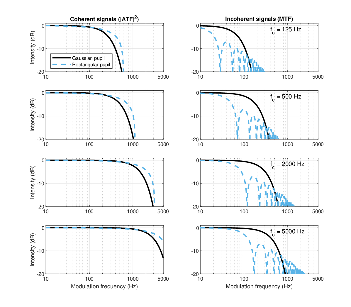
Figure 13.1: Estimated amplitude and modulation transfer functions of the human auditory system, with Gaussian and rectangular pupils and with ideal sampling, at 125, 500, 2000, and 5000 Hz carriers. For coherent inputs (plotted on the left), the modulus square of the ATF is computed, to obtain an intensity measure that is comparable to the incoherent MTF (right). The rectangular-pupil response (dashed blue) is broader than the Gaussian-pupil (solid black) for coherent inputs, but it is much narrower than the Gaussian for incoherent inputs. Additionally, the sinc function (Eq. 13.43) makes the incoherent rectangular-pupil response oscillate many times before it completely decays.

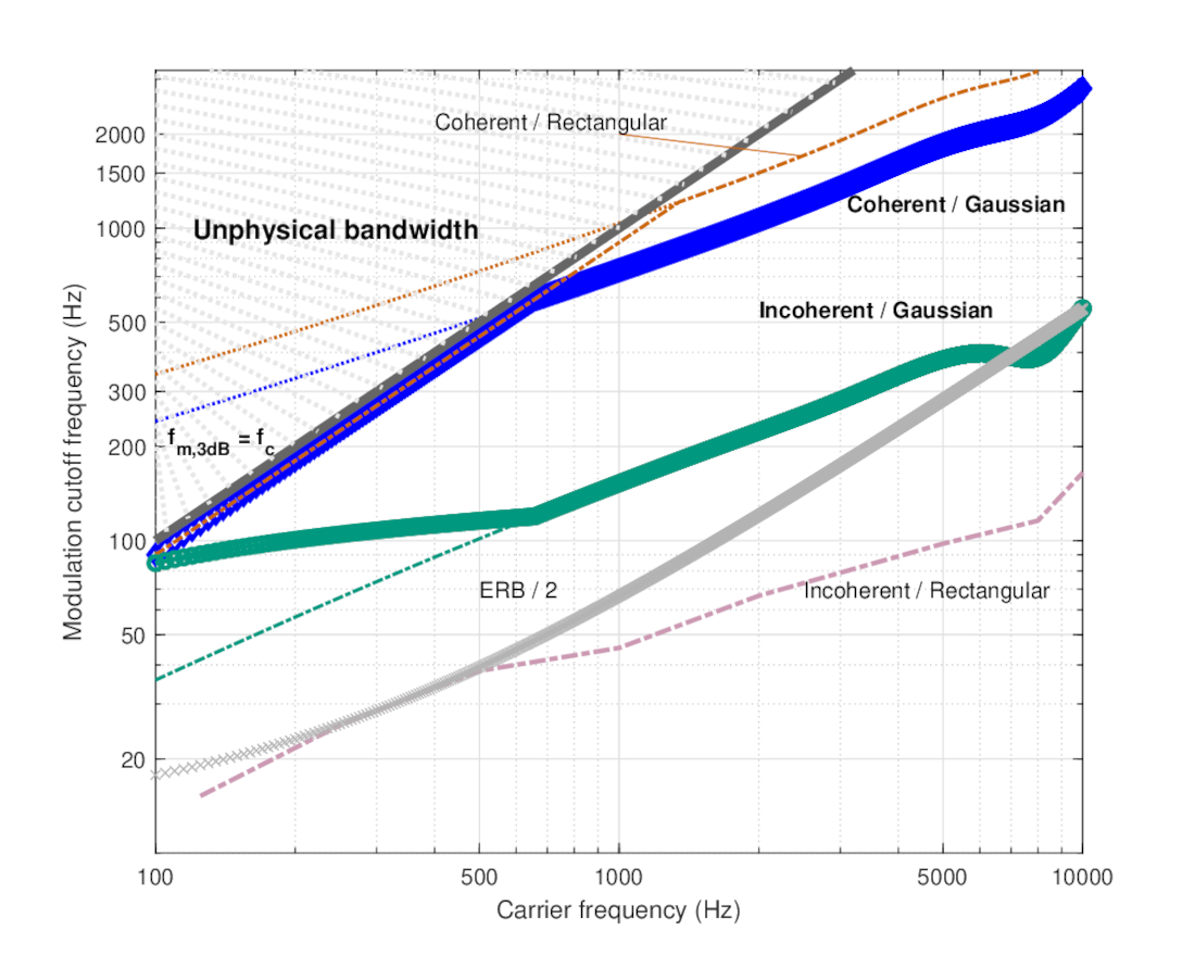
Figure 13.2: The 3 dB cutoff frequencies of the ideal modulation transfer functions with Gaussian and rectangular pupils. The coherent and incoherent Gaussian modulation bandwidths are plotted in thick blue and green lines, respectively. However, if left uncorrected, the original cutoff frequencies would be broader than the carrier, which is physically impossible (the limit \(f_m=f_c\) is in dash gray and the corresponding unphysical area is hatched above it). Using a maximum bandwidth that is somewhat arbitrarily set to \(0.9f_c\), the coherent correction takes place below 660 Hz. For comparison, the responses of rectangular apertures are plotted as well. The coherent rectangular bandwidth (dash-dot red) is \(\sqrt{2}\) larger than the Gaussian, based on Eqs. 13.52 and 13.54. For incoherent modulation, the rectangular bandwidth is 3.37 times narrower than the Gaussian bandwidth (purple dash-dot). The cutoff was computed numerically for the rectangular pupil and according to Eq. 13.53 for the Gaussian. For comparison, the growth of half the auditory filter bandwidth (equivalent rectangular bandwidth, ERB) is plotted in gray crosses (Eq. §11.17), based on Glasberg and Moore (1990).

13.4.2 Empirical TMTF data from literature

With the theoretical MTFs now available, we would like to compare their predictions to empirical data. The dependent variable in behavioral data of the TMTF is the hearing threshold needed for detection of the standard amplitude modulation (AM) signal,

\[ a(t) = \left[ 1 + m \cos(\omega t) \right] \sin(\omega_c t) \,\,\,\,\,\,\,\,\, 0 \leq m \leq 1 \]

(13.55)

as a function of the modulation frequency \(\omega\) and carrier frequency \(\omega_c\), when the carrier is tonal. The modulation depth \(m\), which is equivalent to contrast, is expressed in dB, where \(m=1\) is considered 100% modulation depth. In behavioral studies, the TMTF is tested as a detection threshold—sensitivity to any modulation. Thus, it does not give information about whether the listener hears the particular modulation frequency, or something else. We will return to this subtle point later. In physiological studies of the brainstem and midbrain, the stimulus is usually in full modulation, and the sensitivity is quantified using the synchronization strength to the envelope, producing a TMTF as a function of modulation frequency (Joris et al., 2004).

Several published TMTF curves of different types are compiled in Figure 13.3 and will serve as a reference in the subsequent analysis with several subsets of these curves presented later. As the curves represent thresholds and not sensitivities, they are plotted upside-down compared to the MTFs. The lowest threshold (most sensitive) is rarely lower than about -30 dB. The lowest value should be compared to the 0 dB passband level of the theoretical MTFs, which do not account for internal noise in the auditory system. Therefore, the most, or perhaps the only, relevant parameter of the TMTF that can be compared with the MTF prediction is the cutoff frequency.

At first glance, the theoretical values we obtained for the cutoff frequencies for both pupil functions (Figure 13.2) appear completely at odds with much of the human and animal behavioral TMTF data of Figure 13.3, which show a much narrower modulation bandwidth. This is most readily seen in data using the 5 kHz carrier, which has probably been the most tested frequency of the human TMTF. The 3 dB cutoff frequency was estimated to be anywhere from 144 to 229 Hz for 5 kHz tonal carriers (Stellmack et al., 2005). Additionally, narrowband data exhibit altogether different TMTF morphology, as it has higher threshold at low modulation frequencies—a departure from pure tone TMTFs, which behave like a typical low-pass filter. At high frequencies, the threshold drops again, as the input is spectrally resolved and the modulation can be also detected by adjacent auditory channels, producing a sensitivity that cannot be temporally achieved by a single channel.

All in all, there is a substantial discrepancy between the idealized predictions and the empirical data. While not displayed, it is observed that it is impossible to straightforwardly tweak the imaging parameters—mainly \(v\) and \(T_a\)—to retain consistent results of the temporal resolution and phase curvature data of the previous sections, along with the empirical TMTF data. Therefore, any discrepancy with the empirical data is not only due to misestimation of the dispersion parameters. However, in order to account for this discrepancy, a more detailed analysis of the empirical data is first provided for tonal (coherent) and broadband (incoherent) in the next two subsections. The narrowband data will be used to usher in the discussion about partial coherence in the next section. All together, these analyses will provide some of the necessary insight for the understanding of the role of the auditory defocus.

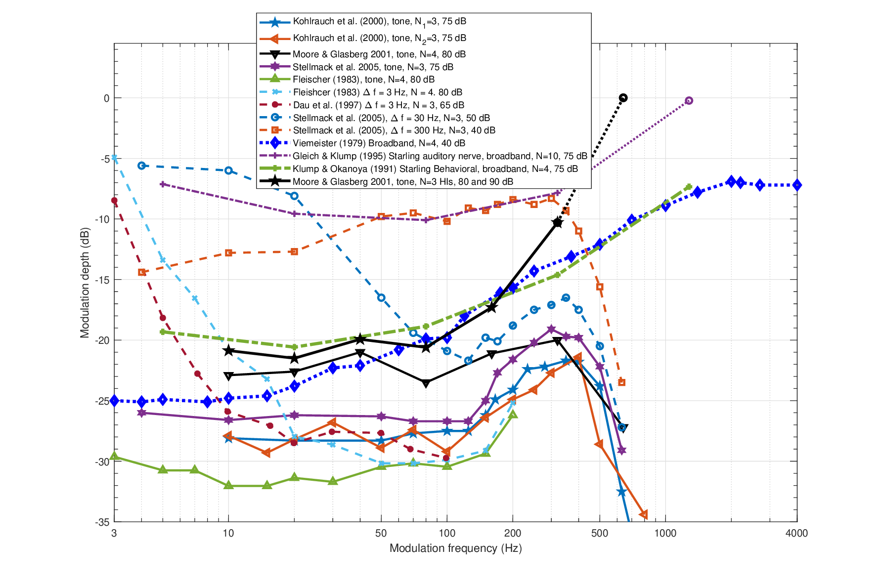
Figure 13.3: Various temporal modulation transfer functions (TMTFs) from literature. Pure tone and narrowband data have all been measured with a 5 kHz carrier, which is therefore the most readily comparable frequency and the only one displayed for tonal and narrowband carriers. The threshold is given in amplitude modulation depth dB (\(20\log m\)), where 0 dB designates 100% modulation (\(m=1\)) in Eq. 13.55. The data were usually collected using a small number of subjects (\(N\)), which is noted in the corresponding legend, along with the type of signal. The curves include two datasets from Kohlrausch et al. (2000, Figures 2 and 3), which were measured with different modulation frequencies and were separated to two groups of three subjects; normal hearing and hearing-impaired tonal data from Moore and Glasberg (2001, Figures 2 and 3); tonal and narrowband data (\(\Delta f = 30,\,\, 300\) Hz) from Stellmack et al. (2005, Figure 3, top right), which reproduced very closely the main observations (but over an extended frequency range) of Dau et al. (1997a, Figures 4–5) with \(\Delta f = 31,\,\, 314\) Hz that are therefore not plotted here; tonal and narrowband data from Fleischer (1983, Figure 1); narrowband data from Dau et al. (1997a) of \(\Delta f = 3\) Hz; broadband data from Viemeister (1979, Figure 2). Finally, two animal broadband datasets are presented of the European starling as measured directly from the auditory nerve (Gleich and Klump, 1995) and behaviorally (Klump and Okanoya, 1991)—both curves were extracted from Figure 9A in Gleich and Klump (1995). Note that at 1280 Hz, there was no measurable physiological response in the starling even at \(m=0\), which is therefore plotted in dotted line and a circle instead of a cross.

13.4.3 Tonal TMTFs

Pure tones are the ultimate coherent carrier and as such should theoretically reflect the low-pass behavior of the coherent auditory ATF. When the pure tone is amplitude-modulated at high enough a frequency, its sidebands are resolved by the adjacent filters. Therefore, with low- and mid-frequency carriers, the low-pass characteristics of the TMTF may not be easily observed, because the modulation is spectrally detected by other channels before the threshold drops, which results in a flat response. At 5 kHz, the equivalent rectangular bandwidth (ERB; Eq. §11.17) is 565 Hz (Glasberg and Moore, 1990), so usually some threshold increase can be observed before it drops again when the sidebands are resolved, as can be seen in Figure 13.3.

The tonal TMTF curves from Figure 13.3 are replotted in Figure 13.4, where the responses are truncated at \(\mathop{\mathrm{ERB}}/2 \approx 283\) Hz, for clarity, just when the threshold is at its highest. All datasets except for those from Moore and Glasberg (2001) show a sharp bend at around 150 Hz, and a cutoff at slightly higher frequency. The normal hearing data from Moore and Glasberg (2001) is inconsistent with these trends, showing a nearly flat response below the half-ERB frequency. However, additional data of three hearing-impaired subjects—likely with broadened auditory filters—revealed a distinct low-pass filter response with a similar cutoff (160 Hz), and no response at 640 Hz modulation. Two subjects had similar responses at 2000 Hz as well, which are not displayed¹²⁸.

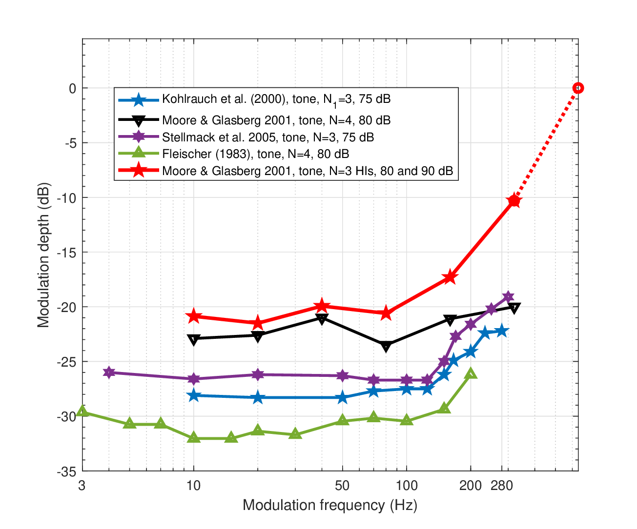
Figure 13.4: A subset of tonal TMTFs at a carrier of 5 kHz. Refer to Figure 13.3 for details. Note that no response could be measured at 640 Hz with the hearing-impaired subjects, even at 100% modulation depth (Moore and Glasberg, 2001). The curves were truncated before the sidebands are spectrally resolved by the adjacent filters, in order to show only the monotonically decreasing responses associated with a single channel.

Regardless of the specific cutoff frequency of the low-pass modulation filter, it is almost an order of magnitude lower than the ideally-sampled coherent ATF that was obtained earlier (about 2 kHz for a 5 kHz carrier, Figure 13.1, bottom left). Therefore, comparison to within-channel auditory nerve measurements may be more revealing than behavioral measurements. For instance, the bandwidth of the cat's auditory nerve TMTF increases to a maximum of about 1500 Hz (Joris and Yin, 1992; Figures 11 and 14). For carriers below 10 kHz, the modulation frequency scales with the carrier and the cutoff frequency reaches a maximum of 1300 Hz. At high tonal carriers it levels off and reaches the absolute maximum at a carrier of 27 kHz. However, several instances of maximum modulation cutoff frequencies that are even higher (1500–2500 Hz) were recorded in the auditory nerve of the cat for carriers between 10 and 30 kHz (Rhode and Greenberg, 1994; Figure 13). Given the high variability in the data and that it may be constrained by physiological limitations on the firing rates and nonexistent phase locking at these carrier frequencies, it is difficult to directly compare these cat data to our predictions. Nevertheless, our very high cutoff prediction (2000 Hz for carrier of 4000 Hz and 3000 Hz for a carrier of 10000 Hz, Figure 13.2) may be more relevant to the specific channel, which carries “pre-perceptual” information that is partially lost on the way downstream (Weisser, 2019).

13.4.4 Broadband TMTFs

Broadband carriers in the audible spectrum represent incoherent signaling and is thus suitable to be tested vis-à-vis the ideal MTF, which predicts a lower cutoff frequency than the coherent ATF, due to defocus. However, the fact that full-spectrum white noise simultaneously excites multiple channels complicates the analysis. It can been dealt with either by filtering out part of the signal, or by combining several auditory-channel-wide stimuli that together produce the broadband stimulus bandwidth. There is an important caveat to this, though—it is not obvious that an auditory-channel-wide white noise signal may be considered a true incoherent carrier, in a sense that is equivalent to complete incoherence in optics, which has vanishingly small coherence time (Eq. §8.31; see also §9.9.2). The frequencies associated with electromagnetic coherence theory are many orders of magnitude larger than the audible range, so that the normal bandwidth of quasi-monochromatic light can have a true randomized phase that covers its entire modulation bandwidth and accrues over numerous periods over short physical distances (Tarnoczy, 1965; originally commented about ultrasound frequencies, which are less affected by this problem than audio frequencies). This means that true incoherent light need not interact with the carrier bandwidth or violate the narrowband assumption. It does not appear to be exactly the case in narrowband sound. While seemingly a technical point, it is nevertheless of great importance, as will be argued below.

Four broadband curves are plotted in Figure 13.5. The most well-known TMTF of sinusoidally modulated white noise was measured by Viemeister (1979) and unlike the tonal TMTFs, it is monotonically rising with a low-frequency cutoff of approximately 40 Hz (compared with about 150–200 Hz in the tonal case at 5 kHz). While a lower cutoff frequency is expected from the general relation between the defocused coherent and incoherent transfer functions (Figure 13.1), it is not obvious how the auditory filter outputs are combined to yield this broadband threshold.

Some insight may be garnered from animals that were tested using comparable stimuli. Observations of the European starling are particularly revealing, because they were obtained both behaviorally (Klump and Okanoya, 1991) and physiologically (Gleich and Klump, 1995). The behavioral starling data follow the human data very closely for modulation frequencies above 80 Hz (green dash-dot curve in Figure 13.5). In contrast, the response to the same stimulus measured in single units of the auditory nerve has a very similar shape, but at a 7–10 dB reduced sensitivity (purple dash-dot curve). Now, returning to human behavioral data, a narrowband carrier of 300 Hz bandwidth produced a threshold that is identical to the starling's auditory nerve at (roughly) 80–320 Hz. Above 320 Hz, the two thresholds diverge, as the human auditory system appears to resolve the narrowband noise, or at least it has access to spectral cues from adjacent filters that reduce the threshold. Hence, it seems that pooling modulation information across fibers can reduce the TMTF threshold in both humans and starlings. Note that additional behavioral data from other animals suggest that the overall threshold (its most sensitive portion) can vary between species (Dent et al., 2002; Figure 4 and Klump and Okanoya, 1991; Figure 5).

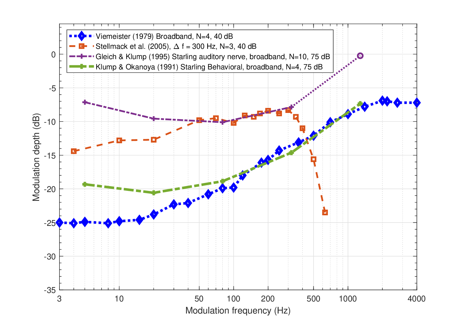
Figure 13.5: Broadband TMTFs. Refer to Figure 13.3 for details.

Assuming that the single-unit starling response to broadband sound does indeed qualify as completely incoherent, it is possible to test it against the ideal-sampling MTF. As we do not have the imaging parameters of the starling system, we can make use of the incoherent temporal acuity expression of Eq. §15.1 that will be introduced in §15.6. Combining it with the expressions for the incoherent cutoff frequency of Eq. 13.53 and the coherent Gaussian-pupil cutoff of 13.52, the following expression is obtained after some algebraic manipulation

\[ f_{inc} = \frac{4 \ln2}{\sqrt{2}\pi} \cdot \frac{1}{d} \approx \frac{0.624}{d} \]

(13.56)

that ties together the temporal acuity \(d\) and the incoherent cutoff frequency \(f_{inc}\) of the MTF. Interpolation of the starling neural TMTF curve in Figure 13.5, sets the 3 dB cutoff at 365 Hz (the curves were averaged over 30 units with CFs between 200 and 3500 kHz, Gleich and Klump, 1995, Figures 6 and 7a). Single-unit auditory nerve broadband gap detection measurements of the starling identified an absolute minimum of \(d=1.6\) ms (at CF = 1.3 kHz, Klump and Gleich, 1991, Figure 4a). Assuming that the minimum gap is achieved with ideal sampling allows us to estimate that \(f_{inc} = 390\) Hz—a fairly close result to \(f_{inc} \approx 365\) Hz (re 80 Hz) from the auditory nerve TMTF measurement from Gleich and Klump (1995) (dash-dot purple in Figure 13.5). In contrast, the behavioral broadband starling cutoff is only 150–180 Hz (Klump and Okanoya, 1991)—about half of the physiological bandwidth. However, linking these physiological and behavioral TMTFs requires consideration of the additional processing stages following the auditory nerve, as well as adequate translation to human hearing.

Two studies directly compared the behavioral and the physiological tonal and broadband TMTFs in the same animals and recording sites. In both studies, the TMTFs were obtained from the inferior colliculus (IC), where the maximum cutoff frequencies observed are expected to be lower than those found the brainstem. Multi-unit recordings of amplitude modulated noise and tonal carriers were compared to behavioral responses of the awake budgerigar (an Australian parrot), whose hearing and vocalization capabilities resemble those of humans (Henry et al., 2016), and in rabbits that have higher thresholds than humans (Carney et al., 2014). In the budgerigar, lower noise-carrier TMTF cutoffs were shown in IC neurons that exhibited higher peak synchrony and higher best modulation frequencies for tonal carriers (Henry et al., 2016; Figure 5). Additionally, for the noise carrier, both the across-channel pooled rate and neural synchrony thresholds were less sensitive to high modulation frequencies (256–512 Hz) and showed no best modulation frequency neurons that are tuned to 512 Hz—the only frequency band measured above 256 Hz (Henry et al., 2016; Figure 7). Very similar results were shown in the rabbit—only less sensitive overall (Carney et al., 2014). In comparison with the budgerigar's data, the cutoff of the ideal Gaussian-pupil incoherent MTF of Figure 13.2 increases slowly with carrier frequency, but also never goes beyond 400 Hz, and even this bound is likely to be reduced by the time it reaches the IC, as was seen in the starling data in §13.4.4. Notably, in both animal studies, both rate and envelope synchrony information was recorded separately and was associated with behavioral performance in the rabbit (spiking rate) and budgerigar and human (synchrony). This observation may suggest that different animals may employ different detection methods to process the modulated sound. While this separation to two coding regimes is commonly employed, they should be both understood as two complementary and indispensable aspects of sampling. If sampling is precise, it must be synchronized to the envelope at an appropriate rate. Otherwise, it necessarily generates sampling errors.

The incoherent-broadband prediction seems to be much more realistic than the coherent predictions for the tonal data, in terms of the modulation bandwidth. Nevertheless, even for the incoherent TMTF, the drop in rate between the physiological and behavioral animal data is substantial. Possible causes for these differences are discussed in §14.8.

13.4.5 Narrowband TMTFs

Narrowband stimuli reveal a range of TMTF responses that are a hybrid of the tonal and the broadband responses, but are neither. Typically, in order to measure the narrowband TMTF, full-spectrum white noise is bandpass-filtered around the carrier and then sinusoidally amplitude-modulated¹²⁹. Because of the relative and absolute proximity of the modulation and the carrier frequency bands, the stochastic carrier bleeds into the lowest frequencies in the modulation band, in proportion to the bandwidth of the carrier¹³⁰. This results in considerable modulation masking energy at low modulation frequencies, which steers the TMTF away from its typical low-pass filter behavior.

Consider the five TMTF curves that are replotted in Figure 13.6. Pure tone modulations elicit the flattest and most sensitive responses. The tonal data by Stellmack et al. (2005) provide the widest frequency range that includes the usual low-pass response before the sidebands are resolved and the threshold drops again beyond the half-ERB frequency. The tonal data by Fleischer (1983) are a bit more sensitive, but are identical in shape. This tonal TMTF was measured in the same setup along with a 3 Hz narrowband carrier TMTF. The tonal and narrowband responses diverge below 50 Hz, but then merge and become indistinguishable (very similar data are given in Dau et al., 1997a; Figure 3, where the responses merge already at 15 Hz). As the narrowband bandwidth broadens (measured for 30 and 300 Hz bandwidths), the responses diverge from the tonal TMTF by becoming less sensitive over a wider modulation bandwidth. The 300 Hz bandwidth curve is much flatter than the 3 and 30 Hz curves, presumably due to the triangular distribution of the modulation spectrum that gets flatter with increased bandwidth (Dau et al., 1997a). As was noted in the broadband TMTF analysis, in the limit of broadband stimuli (Viemeister, 1979), the response shape is about the same as the 300 Hz narrowband, but the sensitivity improves by about 10 dB and continuously decreases, instead of being resolved by adjacent filters.

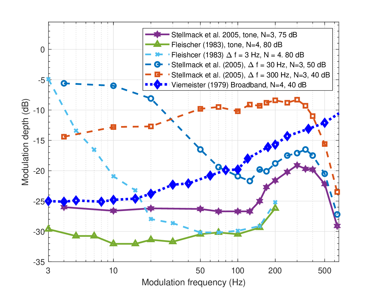
Figure 13.6: Narrowband TMTFs. Refer to Figure 13.3 for details.

It is apparent that the responses generated by the narrowband stimuli are not well-described by either coherent or incoherent MTFs. This type of signals requires the much more general framework of partial coherence, which better taps realistic signals as well. It is discussed below.

13.5 Modulation and partially coherent sound

The partial overlap between the narrowband and tonal TMTFs reveals a great deal about the auditory system sensitivity to carrier types. A narrowband carrier—even if stochastic by design—cannot be considered truly incoherent if it contains discernible modulation components that compete with the target modulation. Moreover, as it becomes indistinguishable from a fully coherent carrier at higher modulation frequencies, it may have effective qualities of a coherent carrier. If this is correct, then narrowband carriers such as the 3 Hz and the 30 Hz bandwidths from Figure 13.6 should be able to interfere and beat together, even though they are not tonal. This should not be surprising, as both coherence time and length—the measures of the degree of coherence over time and space, respectively—are inversely proportional to the bandwidth of the carrier (§8.2.4). So, by definition, a pure tone has a degree of coherence of 1, white noise 0, and narrowband signal somewhere in between. It was also shown how the filter bandwidth in which sounds are analyzed can increase the apparent coherence of otherwise incoherent signals, even if they never become exactly the same (§8.2.8). Either way, the compiled data of tonal, broadband, and narrowband TMTFs strongly suggest that narrowband sounds may be best understood as partially coherent, rather than completely incoherent.

To illustrate the partial coherence of narrowband sounds, the beating of two narrowband sounds with different bandwidths is visualized in Figure 13.7 using one-dimensional and monochromatic interference patterns, or interferograms. Additionally, the effective amplitude modulation of three narrowband sounds (carrier plus two sidebands) is shown in Figure 13.8. The interferograms are particularly descriptive in illustrating the basic measure of interference that is fundamental in imaging as well—visibility or contrast (i.e., modulation depth)—which is not as vividly represented in normal time signal plots. Unlike optical interferograms, the x-axis represents time instead of a static spatial dimension. The plot height contains no information and is used only for visualization. Audio demos corresponding to the two figures are found in /Section 13.5 - Modulation and partially coherent sound/.

In Figure 13.7, the interference of two narrowband sounds of bandwidth \(\Delta f_c\) and frequency spacing \(\Delta f\) is shown. After demodulation, the beating between the components at frequency \(f_c \pm \Delta f/2\) translates to \(\Delta f\) in the intensity pattern, which was obtained after low-pass filtering the carrier and squaring. In the top row of the figure, \(\Delta f_c = 0\), which is the classical beating of two pure tones for three different frequency separations \(\Delta f\) of 4, 10 and 40 Hz, over 1 s duration. The interference patterns are fully periodic and exhibit high contrast between the peaks and the troughs, showing as completely black background. In the next three rows, three narrowband carriers with \(\Delta f_c\) of 2, 20 and 100 Hz are interfered for the same spacing. As the bandwidth of the carrier increases, the image becomes gradually irregular, the periodicity is disrupted, and the contrast is lost, so the interference pattern turns more uniform, on average.

The loss of contrast is more apparent in the second set of interferograms in Figure 13.8, which illustrates AM interferences between a narrowband carrier and two narrowband sidebands. The loss of contrast is most apparent in the second row. As three sounds with random phase interfere here, the coherent-looking patterns are visible only for the carrier with 2 Hz bandwidth, where the modulation frequency and carrier frequency appear superimposed. For larger bandwidths, the patterns no longer show visible interference and the modulation rate sounds almost unrecognizable. Thus, the degree of coherence for such an AM stimulus is smaller than the beating source. Note that if the sidebands would have been produced directly using a sine function instead of narrowband sidebands, then the interference would have been much stronger and closer to the results from literature.

In these examples, the effect of the auditory filter itself was not taken into account, but the corresponding perceptual effects can be heard in the supplementary sound demos. The interference between narrowband noise maskers and narrowband noise or pure tone targets and the likely effect of beating has been occasionally discussed in literature. See for example, Egan and Hake (1950) and Moore et al. (1998).

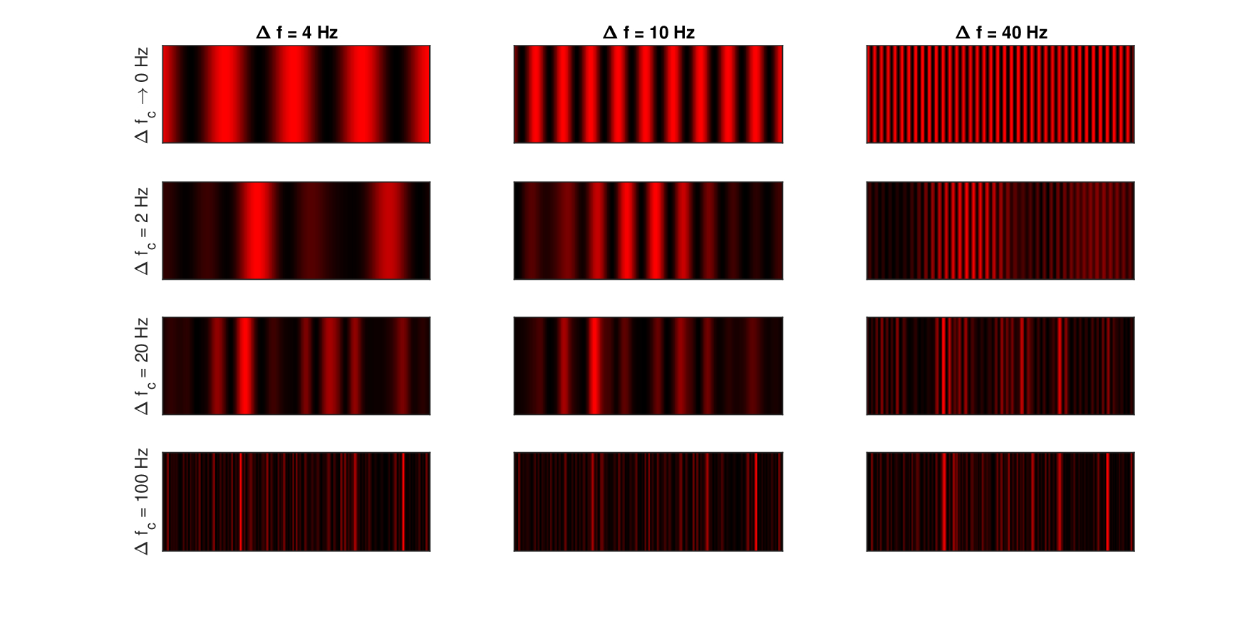
Figure 13.7: The interference caused by beating of two tones (top row) or narrowband sounds (bottom three rows). The patterns were generated by summing two time signals centered at \(f_c = 5\) kHz of bandwidth \(\Delta f_c\) that are separated by \(\Delta f\), squaring them, and low-pass filtering the output using a fourth-order Butterworth filter with 400 Hz cutoff. The top row is the interference pattern of two pure tones, with no random components. The duration is always 300 ms. Narrowband carriers were generated by zeroing the out-of-band frequencies from the Fourier transform of broadband Gaussian white noise signals, as in Dau et al. (1997a). The output is mapped to 256-level intensity color map.

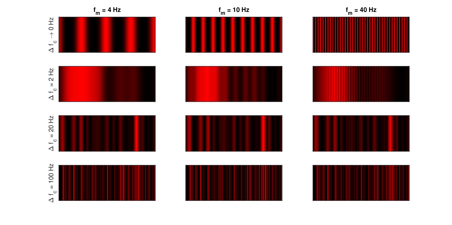
Figure 13.8: The interference caused by amplitude modulation of pure tones (top row) or narrowband sounds (bottom three rows). The patterns were generated by summing three time signals centered at \(f_c = 5\) kHz and \(f_c \pm f_m\) at half the carrier level, with additional details identical to Figure 13.7.

13.6 Discussion and conclusion

In this chapter we derived the various impulse response functions for the human auditory system, as well as its modulation domain transfer functions. These functions bring to light the significance of the defocus in the system, as it differentiates the coherent and incoherent signal regimes that enter the system.

We compared the predictions from this theory in terms of MTF bandwidth to human data of broadband, tonal, and narrowband TMTFs. That there are significant differences between the functions that could be predicted from theory, but the actual bandwidths were grossly overestimated when compared to behavioral thresholds and only roughly corresponded to single-channel measurements from the auditory nerve of animals. This discrepancy is puzzling given the robust prediction we obtained in the time-domain analysis in §12.4 using the very same parameters. As will be shown in the next chapter, this can be explained by incorporating sampling into the system, which is known to degrade the spatial MTF of light in optics.

Despite the discrepancy in the TMTF and predicted MTF, the intuition that is garnered by the idealized frequency-domain analysis will remain valuable in the chapters to come. Namely, coherent signals have broader modulation bandwidth than incoherent signals, due to the inherent defocus of the auditory system that differentiates the ATF and the MTF. For this conclusion to be meaningfully used, the concept of partial coherence must be considered in the analysis of typical auditory stimuli. It should be emphasized, though, that the sensed coherence is not necessarily equal to the stimulus coherence. The sensed degree of coherence of the source is directly tied to the filter bandwidth that processes the signal and on the ensuing phase locking provided by the system. These factors will be discussed in §16.4 in the context of auditory accommodation.

Using the modulation spectrum analysis, we obtained two further insights about the temporal aperture of the system. First, its pupil function is indeed closer to a Gaussian than to a rectangular window, in line with animal data from the chinchilla, and earlier results in §12.5. Second, at low frequencies, the aperture stop is likely be the result of the cochlear filters, perhaps combined with other elements, rather than the neural spiking that dominates the high frequencies. This justifies the correction to the aperture time values that was required to account for the low-frequency cochlear phase curvature prediction data in §12.5.

Footnotes

123. See the appendix in Jiang et al. (2013) for a derivation of a similar two-dimensional OTF.

124. In hearing, this envelope is represented by beating, where we do not hear any difference between the negative and positive modulation half cycles, which amounts to an effective period doubling. In contrast, classical amplitude modulation (with envelope of the form \(1+ m \cos(\omega_m t)\)) has a linear component as well that is directly associated with \(H(\omega_m)\). The simple trigonometric identity underlying it may be also explained more intuitively using sampling theory and is revisited in §E.

125. The perfect-sampling condition allows us to interpret the continuous signal expressions at face value. This condition will be relaxed later, as evidence will emerge that can be interpreted as suboptimal sampling that degrades the various MTFs.

126. As the Gaussian pupil function is real, its OTF is always positive, which makes it identical to the MTF. Therefore, we will refer to it as MTF, to suggest similarity to the TMTF and simplify the terminology going forward. However, in the case of the rectangular pupil, the OTF changes signs, so a distinction will be made between the OTF and MTF.

127. The modulation filters were characterized by the cutoff frequency, which is where the synchronization coefficient drops to 0.1 and is therefore higher in frequency than the 3 dB cutoff (Rhode and Greenberg, 1994; Figure 1).

128. Few other studies are also inconsistent with the low-pass response and tend to show bandpass behavior at very low frequencies (e.g., Yost and Sheft, 1997). These effects may be related to signal presentation methods and to longer temporal integration effects that are beyond the scope of this analysis. See Kohlrausch et al. (2000) for further discussion.

129. The order of the bandpass filtering and modulation operations was not the same in different studies, but was shown to elicit very similar TMTFs (Dau et al., 1997a; Stellmack et al., 2005). It appears that the two orders produce responses that are close enough both qualitatively and quantitatively, so whatever difference exists between the two is ignored in the analysis.

130. Dau et al. (1997a) highlighted that according to a proof by Lawson and Uhlenbeck, 1950, a rectangular carrier envelope in the spectral domain results in a triangular envelope in the spectral modulation domain of the same bandwidth. We saw in §13.3 that this is a general result of the autocorrelation of rectangular windows, only that the resultant bandwidth is doubled. See Dau et al. (1999) for further investigations.

References

Boreman, Glenn D. Modulation transfer function in optical and electro-optical systems, volume TT52. SPIE Press – The International Society for Optical Engineering, Bellingham, WA, 2001.

Born, Max, Wolf, Emil, Bhatia, A. B., Clemmow, P. C., Gabor, D., Stokes, A. R., Taylor, A. M., Wayman, P. A., and Wilcock, W. L. Principles of Optics. Cambridge University Press, 7th (expanded) edition, 2003.

Bour, Lo J and Apkarian, Patricia. Selective broad-band spatial frequency loss in contrast sensitivity functions. Comparison with a model based on optical transfer functions. Investigative Ophthalmology & Visual Science, 37 (12): 2475–2484, 1996.

Carney, Laurel H, Zilany, Muhammad SA, Huang, Nicholas J, Abrams, Kristina S, and Idrobo, Fabio. Suboptimal use of neural information in a mammalian auditory system. Journal of Neuroscience, 34 (4): 1306–1313, 2014.

Dau, Torsten, Kollmeier, Birger, and Kohlrausch, Armin. Modeling auditory processing of amplitude modulation. I. Detection and masking with narrow-band carriers. The Journal of the Acoustical Society of America, 102 (5): 2892–2905, 1997a.

Dau, Torsten, Verhey, Jesko, and Kohlrausch, Armin. Intrinsic envelope fluctuations and modulation-detection thresholds for narrow-band noise carriers. The Journal of the Acoustical Society of America, 106 (5): 2752–2760, 1999.

Dent, Micheal L, Klump, Georg M, and Schwenzfeier, Christian. Temporal modulation transfer functions in the barn owl (Tyto alba). Journal of Comparative Physiology A, 187 (12): 937–943, 2002.

Egan, James P and Hake, Harold W. On the masking pattern of a simple auditory stimulus. The Journal of the Acoustical Society of America, 22 (5): 622–630, 1950.

Fleischer, H. Modulation thresholds of narrow noise bands. In Proceedings of the 11th ICA, Paris, pages 99–102, 1983.

Forrest, TG and Green, David M. Detection of partially filled gaps in noise and the temporal modulation transfer function. The Journal of the Acoustical Society of America, 82 (6): 1933–1943, 1987.

Glasberg, Brian R and Moore, Brian CJ. Derivation of auditory filter shapes from notched-noise data. Hearing Research, 47 (1-2): 103–138, 1990.

Gleich, Otto and Klump, Georg M. Temporal modulation transfer functions in the European Starling (Sturnus vulgaris): II. Responses of auditory-nerve fibres. Hearing Research, 82 (1): 81–92, 1995.

Goodman, Joseph W. Introduction to Fourier Optics. W. H. Freeman and Company, New York, NY, 4th edition, 2017.

Henry, Kenneth S, Neilans, Erikson G, Abrams, Kristina S, Idrobo, Fabio, and Carney, Laurel H. Neural correlates of behavioral amplitude modulation sensitivity in the budgerigar midbrain. Journal of Neurophysiology, 115 (4): 1905–1916, 2016.

Jiang, Xiaoyu, Pei, Chuang, Yan, Xingpeng, Liu, Junhui, and Zhao, Kai. Optimization of exit pupil function: Improvement on the OTF of full parallax holographic stereograms. Journal of Optics, 15 (12): 125402, 2013.

Joris, Philip X and Yin, Tom CT. Responses to amplitude-modulated tones in the auditory nerve of the cat. The Journal of the Acoustical Society of America, 91 (1): 215–232, 1992.

Joris, PX, Schreiner, CE, and Rees, A. Neural processing of amplitude-modulated sounds. Physiological Reviews, 84 (2): 541–577, 2004.

Klump, Georg M and Okanoya, Kazuo. Temporal modulation transfer functions in the European starling (Sturnus vulgaris): I. Psychophysical modulation detection thresholds. Hearing Research, 52 (1): 1–11, 1991.

Klump, Georg M and Gleich, Otto. Gap detection in the European starling (Sturnus vulgaris). Journal of Comparative Physiology A, 168 (4): 469–476, 1991.

Kohlrausch, Armin, Fassel, Ralf, and Dau, Torsten. The influence of carrier level and frequency on modulation and beat-detection thresholds for sinusoidal carriers. The Journal of the Acoustical Society of America, 108 (2): 723–734, 2000.

Kolner, Brian H. Space-time duality and the theory of temporal imaging. IEEE Journal of Quantum Electronics, 30 (8): 1951–1963, 1994a.

Kolner, Brian H. The pinhole time camera. Journal of the Optical Society of America A, 14 (12): 3349–3357, 1997.

Lawson, James L. and Uhlenbeck, George E. Threshold Signals. McGraw-Hill Book Company, Inc., 1950.

McCluney, William Ross. Introduction to Radiometry and Photometry. Artech House, Inc., Norwood, MA, 1994.

Moore, Brian CJ, Alcántara, Joseph I, and Dau, Torsten. Masking patterns for sinusoidal and narrow-band noise maskers. The Journal of the Acoustical Society of America, 104 (2): 1023–1038, 1998.

Moore, Brian CJ and Glasberg, Brian R. Temporal modulation transfer functions obtained using sinusoidal carriers with normally hearing and hearing-impaired listeners. The Journal of the Acoustical Society of America, 110 (2): 1067–1073, 2001.

Oxenham, Andrew J and Dau, Torsten. Towards a measure of auditory-filter phase response. The Journal of the Acoustical Society of America, 110 (6): 3169–3178, 2001a.

Park, Stephen K, Schowengerdt, Robert, and Kaczynski, Mary-Anne. Modulation-transfer-function analysis for sampled image systems. Applied Optics, 23 (15): 2572–2582, 1984.

Recio-Spinoso, Alberto and Oghalai, John S. Mechanical tuning and amplification within the apex of the guinea pig cochlea. The Journal of Physiology, 595 (13): 4549–4561, 2017.

Recio-Spinoso, Alberto and Oghalai, John S. Unusual mechanical processing of sounds at the apex of the guinea pig cochlea. Hearing Research, 370: 84–93, 2018.

Rhode, William S and Greenberg, Steven. Encoding of amplitude modulation in the cochlear nucleus of the cat. Journal of Neurophysiology, 71 (5): 1797–1825, 1994.

Schroeder, Manfred R. Modulation transfer functions: Definition and measurement. Acta Acustica united with Acustica, 49 (3): 179–182, 1981.

Stellmack, Mark A, Viemeister, Neal F, and Byrne, Andrew J. Monaural and interaural temporal modulation transfer functions measured with 5-khz carriers. The Journal of the Acoustical Society of America, 118 (4): 2507–2518, 2005.

Tarnoczy, T. Sound focussing lenses and waveguides. Ultrasonics, 3 (3): 115–127, 1965.

Van Nes, Floris L and Bouman, Maarten A. Spatial modulation transfer in the human eye. Journal of the Optical Society of America, 57 (3): 401–406, 1967.

Viemeister, Neal F. Temporal modulation transfer functions based upon modulation thresholds. The Journal of the Acoustical Society of America, 66 (5): 1364–1380, 1979.

Weisser, Adam. Auditory information loss in real-world listening environments. arXiv preprint arXiv:1902.07509, 2019.

Wittenstein, W, Fontanella, JC, Newbery, AR, and Baars, J. The definition of the OTF and the measurement of aliasing for sampled imaging systems. Optica Acta: International Journal of Optics, 29 (1): 41–50, 1982.

Yost, William A and Sheft, Stanley. Temporal modulation transfer functions for tonal stimuli: Gated versus continuous conditions. Auditory Neuroscience, 3: 401–414, 1997.

de Luca, Luigi and Cardone, Gennaro. Modulation transfer function cascade model for a sampled IR imaging system. Applied optics, 30 (13): 1659–1664, 1991.