Chapter 14

The use of sampling for imaging continuous signals

14.1 Introduction

The visual image consists of relatively static frames that are perpetuated in time, which is then perceived as a degenerate dimension of the object. Such images can be thought of as time-independent, as they represent spatial patterns that appear to be frozen in time. Visible temporal changes in the spatial image often require macroscopic movement to take place. It is mapped to an extra dimension and requires sequential imaging that is continually refreshed. The same holds also in the case of still and moving-image cameras. Both devices contain almost the same optics, but only the latter has an explicit added dimension of time and, hence, movement.

In contrast to light that is produced by quantum processes on the atomic and molecular levels, sound production requires continuous macroscopic movement (vibration), whose temporal dependence is much closer to relevant biological time constants than light, by many orders of magnitude. The way that the auditory system is designed to receive the signals confines them to being spatially one-dimensional, which means that all temporal and spatial dependencies are mathematically projected on a one-dimensional audible time signal. This means—to complete the analogy with vision—that a static image of a pulse, or part thereof, must be taken as a stepping stone to a continuous image of moving objects. Unlike photography though, sound recording is only interesting inasmuch as it can capture “moving” sound, and not just a single pulse. Therefore, the concept of an “acoustic still shot” is of little use outside of theoretical research.

Acoustic signals are generally continuous, whereas the various expressions developed in the temporal imaging theory relate to pulses. In fact, nowhere in the temporal imaging equations is it made explicit that the envelopes must be shaped as pulses to satisfy the imaging operation. By the physical nature of the system, it has a finite temporal aperture, which represents what the system can “see” at any one time. Through modeling the psychoacoustic phase curvature data using the continuous temporal imaging equations, it became abundantly clear in §12.4 that the system has a finite aperture. A finite aperture was then included in the impulse response and modulation transfer functions, as the defining feature of the pupil function (§13.2). Effectively, it is this aperture that imposes a pulse shape on the incoming signal—it is not necessary for the signal itself to enter the system in a pulse form.

In this chapter we will integrate some of the most elementary principles of sampling theory into the auditory temporal imaging theory. Auditory sampling, which happens in the transduction of the auditory nerve and in all subsequent synapses, is nonuniform and extends to a finite duration per sample, unlike classical sampling techniques. The implications will be discussed, mainly with respect to the narrowing of the temporal modulation transfer function between the periphery and higher auditory areas. An additional discussion about the implications of discrete processing and how it compares with continuous temporal models of hearing is provided in §E.

14.2 Sampling in hearing theory

While sampling is an indispensable operation in modern signal processing that is based on discretized representations of all analog signals, it is not an integral concept in hearing theory itself, although it arguably deals with neurally discretized signal representations. In this brief section, the exceptions to this trend in literature are mentioned—nearly all of which were modeled independently of one another.

In psychoacoustics, two models exist that employ either “looks” (Viemeister and Wakefield, 1991) or “strobes” (Patterson et al., 1992; adopted also in Lyon, 2018)—discrete samples in the auditory signal processing. In some conditions, these models provide better predictions to experimental data than continuous “leaky integration” or “sliding window” models. These models are not given precise physiological correlates, or detailed technical parameters about the sampling. See §E for a further discussion.

Sampling is somewhat more common in physiological models of hearing. Several auditory signal processing models exist that were inspired by nonuniform or irregular sampling of wavelet frames, whose exact physiological correlate is not made explicit (Yang et al., 1992; Benedetto and Teolis, 1993; Benedetto and Scott, 2001).

Most sampling models relate directly to the auditory nerve. Lewis and Henry (1995) and Yamada and Lewis (1999) referred to the noise from the high spontaneous rate auditory nerve fibers as performing dithering¹³¹—a term that is normally used only in the context of sampling and conversion between digital and analog signal representations. A more specific mechanism of sampling was considered by Heil and Irvine (1997) and Heil (2003), where the auditory nerve coding of the onset of temporal envelopes was modeled as equivalent to point-by-point sampling of the envelope function, which tracks it at high resolution, limited by the spike/sampling rate. Another neural processing model makes use of the concept of stochastic undersampling to show how deafferentation of the auditory nerve is analogous to noise (Lopez-Poveda and Eustaquio-Martin, 2013b; Lopez-Poveda, 2014). This model has some parallels to the classical volley principle, whereby the acoustic input is adequately sampled (or even oversampled) by a population of neural fibers, each of which by itself undersamples the signal (Wever and Bray, 1930b; §1.2).

Similar ideas were sometimes attributed to higher-level nuclei such as the brainstem. Warchol and Dallos (1990) suggested that high spontaneous rates in the avian auditory cochlear nucleus enable better sampling of the stimulus. Additionally, Yang et al. (1992) noted that the anteroventral cochlear nucleus (AVCN) receives inputs from the auditory nerve, which could be instantaneously mismatched and then lead to effective lateral inhibition. This perspective may be interpreted as another form of nonuniformity in the sampling that exists beyond the stochastic auditory nerve spiking pattern. Further downstream, Poeppel (2003) suggested that the two auditory cortices work by asymmetrically sampling the incoming sound—the left hemisphere samples the auditory cortex at around 40 Hz, and the right hemisphere at 4–10 Hz. This sampling strategy is thought to be particularly advantageous for speech processing, where information on different time scales can be extracted simultaneously.

Finally, sampling in the spectral domain of the spectral envelope was also considered in the context of a model for vowel identification, which can be degraded when the harmonic content is rich and the fundamental frequency is high, because of spectral undersampling and resultant aliasing distortion (de Cheveignè and Kawahara, 1999). The model was also formulated in the temporal domain using autocorrelation, which may have a physiological correlate. More generally, the model was applied for pitch perception as well (de Cheveigné, 2005).

14.3 Basic aspects of ideal sampling

The temporal imaging theory is based on envelope objects that are shaped as finite pulses. However, realistic signals are long and continuous, so the theory must be extended to include signals of arbitrary durations. A natural solution is to internally construct the signal as a sequence of pulses. Each pulse is an image in its own right, but can also be thought of as a sample. It is possible in general to use the system linearity and time-invariance (only approximate features in our case) to impose the pulse internally and relax the condition that the input is shaped as a pulse. This was demonstrated naturally in our model of the psychoacoustic phase curvature responses, which assumed that the continuous signal is shaped according to the aperture stop of the system. In theory, if the signal is sampled frequently enough, an accurate reconstruction can be made that recovers the complete, arbitrary signal, based on sampling theory. If this happens on multiple channels in parallel, then the complete auditory image can be reconstructed from the individual channel images¹³².

Ideal sampling is represented as a periodic array of delta functions (also called a comb function):

\[ s(\tau) = \sum_{n=-\infty}^{\infty} \delta(\tau-nT_s) \]

(14.1)

with period \(T_s\) that is determined by the sampling rate \(T_s = 1/f_s\). The sampled version of an input \(a(t)\) is then:

\[ a_s(\tau) = \sum_{n=-\infty}^{\infty} a(nT_s) \]

(14.2)

Using Fourier series with period \(T_s\), it is possible to obtain the spectrum of the sampler (see, for example Pelgrom, 2010; pp. 133–136):

\[ S(\omega) = \frac{1}{T_s}\sum_{m=-\infty}^{\infty} \delta(\omega - m \omega_s) \]

(14.3)

And the corresponding spectrum of the sampled signal is

\[ A_s(\omega) = \frac{1}{T_s}\sum_{m=-\infty}^{\infty} A(\omega - m\omega_s) \]

(14.4)

Therefore, the spectrum of the sampled signal is periodic as well and repeats in multiples of \(f_s = \omega_s/2\pi\). As long as the sampled signal is bandlimited and satisfies the Nyquist criterion of \(B < 2f_s\), the periods of the spectrum stay clear of one another and perfect reconstruction of the signal is possible, according to Shannon's sampling theorem (§5.2.1). But if this bound is breached, then the reconstruction will include spectral components that are not in the original input and give rise to aliasing (see an example in Figure 14.1). Therefore, an anti-aliasing (low-pass) filter is commonly employed to ensure that the input to the sampler is bandlimited. The ideally reconstructed signal is then given by

\[ a_s(\tau) = \sum_{n=-\infty}^{\infty} a(nT_s) \mathop{\mathrm{sinc}}\left(\frac{\tau - nT_s}{T_s}\right) \]

(14.5)

In practical engineering designs, a sinc filter is never used, but there are many approximations that can achieve almost as good a reconstruction as this theoretical one (Unser, 2000).

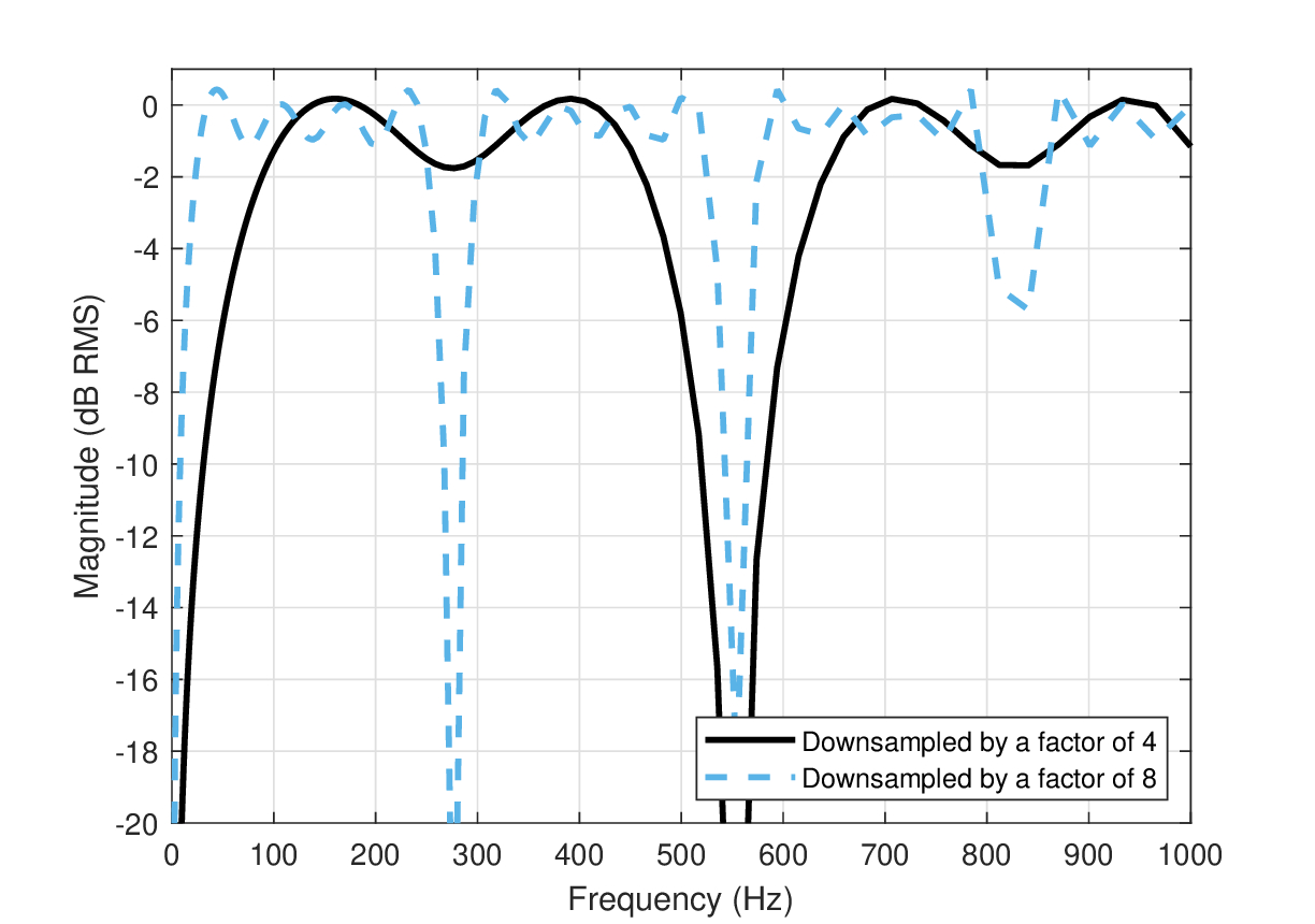
Figure 14.1: The apparent frequency response caused by downsampling a signal when it contains frequencies higher than the Nyquist limit and no anti-aliasing filter is employed. In the examples, sine tones generated at a sampling rate of \(f_s = 4410\) Hz were resampled using delta impulse functions at rates of 1102 Hz (solid black) and 551 Hz (dash blue). All frequencies above half the downsampling rates are aliased products caused by folded tones of lower frequencies. This aliasing gives rise to distinct notches in the frequency response.

14.4 Auditory sampling and imaging

In spatial imaging, the single samples are bits of intensity at a certain wavelength channel, corresponding to color pixels. In vision, photoreceptor activation was shown to occur from single photons (Bialek, 1987). Is the correct way to understand hearing equivalent to vision—point-by-point sampling of the acoustic signal? We shall go over the canonical sampling types to try and shed some light over this question.

14.4.1 Impulse sampling

Impulse sampling is achieved when the sampling windows are infinitesimally short, as each one is well-approximated by a delta function (Couch II, 2013; pp. 93–95; see A and B in Figure 14.2). Obviously, the sampling window always has a finite width, even if it is approximated mathematically as a delta function. Insofar as the entrance pupil that was estimated in §12.5 reflects the sample duration, an infinitesimally short impulse sampling is not supported by the data. In practice, however, the effective pulse must have been represented by a population of neurons in the auditory channel that fired more or less simultaneously. It is possible that each neuron in itself samples the image that we considered as a pulse in the temporal imaging equations. The sampled and coded pulse then propagates downstream, where the impulsive nature of the initial sampling may or may not be perceived. At present, this sampling model cannot be confirmed or rejected.

Figure 14.2: Different sampling types. A: The original signal. B: Impulse sampling. C: Natural sampling. D: Flat-top sampling.

14.4.2 Natural sampling and images

A realistic sampler cannot have infinitesimally short samples, so the delta function should be replaced with a window function, or in our case, with the image of the aperture as it appears on the input—what we referred to earlier as the entrance pupil, \(P_e(\tau)\). Each delta function in the grid of samples, can be therefore replaced with the entrance pupil, which yields

\[ s(\tau) = P_e(\tau) \ast \sum_{n=-\infty}^{\infty} \delta(\tau-nT_s) = \int_{-\infty}^{\infty} P_e(\tau') \sum_{n=-\infty}^{\infty} \delta(\tau -nT_s -\tau')d\tau'\\ =\sum_{n=-\infty}^{\infty} \int_{-\infty}^{\infty} P_e(\tau') \delta(\tau -nT_s -\tau')d\tau'= \sum_{n=-\infty}^{\infty} P_e(\tau-nT_s) \]

(14.6)

And accordingly,

\[ a_s(\tau) = a(\tau) \sum_{n=-\infty}^{\infty} P_e(\tau - nT_s) \]

(14.7)

This turns the continuous object into a periodic sequence of pulses in a shape that is constrained by the duration of the entrance pupil (see §12.5). As is familiar from temporal windowing in signal processing, the shape of the entrance pupil interacts with the output spectrum of the input as well.

When the sample has a finite duration, but it faithfully tracks the signal amplitude while it is on, it is referred to as natural sampling (Couch II, 2013; pp. 133–137; see A and C in Figure 14.2). Once again, the original signal can be reconstructed using the same principles as impulse sampling, but the spectrum depends also on the duty cycle of the sampler—the relative signal duration that is being sampled—in addition to the original spectrum. In our case, we successfully used a Gaussian pupil function, which suggests that the sample is natural, in the sense that it is possibly weighted in amplitude before it is being coded. However, as spikes do not convey amplitude directly (only through their aggregate spiking rate), the concept of weighting may not be necessarily valid on the individual-sample basis.

In two static spatial dimensions, natural sampling is really a complete image, where the sample duration is analogous to the aperture stop. The interesting thing about it is that a natural sample contains much information in itself, unlike the impulse sample that only encodes the amplitude of the signal at one time point. In monaural human hearing, standalone signals that are less than, say, 2–3 ms, do not appear to convey any useful information, so they may not count as anything more than a single data point. This is not the case in echolocating bats (Eptesicus fuscus), though, which were shown to be able to extract information from single reflected pulses that are about 0.4 ms long (the maximum resolution of single pulses), possibly by comparing them to stored signal data. The information contained in that pulse was shown to be discernible by bats with variations of tens of nanoseconds or longer (!) (Simmons et al., 1990; Simmons et al., 1996). While this information may be extracted in different ways (Sanderson et al., 2003), it may attest to that, at least for some mammals, a single pulse might not be just a single data point. In contrast, in humans, all major percepts (e.g., pitch and loudness) are integrated over tens of milliseconds, or longer. A single impulse has no distinct pitch (Doughty and Garner, 1947). At 1 ms or less, only binaural cues are used to determine localization through interaural-time difference, which does not require the detailed information of the sample, but only its onset data or relative phase. Nevertheless, the curvature data extracted in §12.4 was mathematically based on a single sample—a “snapshot” of the periodic chirping masker as it repeatedly crossed the narrowband pure-tone target.

There is another way to look at natural sampling that is rather counterintuitive, if one is primarily used to think of spectral resolution as the main limitation that underlies the auditory system's performance. When high frequency-sensitivity is a critical goal, then the uncertainty principle dictates that the temporal window should be as long as possible to achieve high spectral precision and allow for the output of the slow high-Q bandpass filter to build up. According to this perspective, the identity of the tuned filter discloses the signal frequency, as its only measurable output is signal power at that frequency. However, the temporal aperture itself—which is determined by the bandpass filter of the channel only if it is also the aperture stop—can be also seen as a modulation-band low-pass filter, whose cutoff frequency increases with the window duration (Eqs. §13.52 and §13.53). The auditory temporal aperture used for sampling fulfills an opposite target in the case of impulse sampling, where it has a zero modulation bandwidth that completely excludes any fluctuations, whereas an infinitely long sample would contain all the variations of the object modulation band. Here, the longer the natural sample is, the wider is its passband and more modulation information is preserved in the image. Then, if the passband is too broad, the modulation information may be smoothed if it is carried by too many frequencies that are all averaged together (cf., Oxenham and Kreft, 2014). These reciprocal relations suggest that if natural sampling is relevant in hearing, there may be a trade-off in setting the ideal temporal aperture, modulation bandwidth, spectral bandwidth, and sampling rate of the channel—parameters that are not all independent of one another. See also the discussion in §6.6.2 for a complementary view about the information conveyed by the spectral and modulation spectra.

While the natural sample view is mathematically sound, it is challenging in terms of the underlying neuronal mechanisms that are supposed to sample or communicate such information, as they may have to carry more information than may appear to be borne by a single discharge. As was mentioned in §14.4.1, it could be the result of firing by a few sampling neurons that together combine into a higher-level sample that contain more information. However, given the example of the hyperacute temporal perception of the bat, we should remain open to the conceptually challenging option that a single spike contains more information than a digital sample does in engineered applications. This point of view is currently not supported by neuroscientific theory.

14.4.3 Flat-top sampling

Flat-top sampling is a combination of impulse and natural sampling in that it samples the input signal over a finite duration, in which one level of the signal is recorded (Couch II, 2013; pp. 137–141; see A and D in Figure 14.2). In electronics, this is typically the onset or peak level, using a sample-and-hold circuitry, which makes this popular technique simple to implement. The original spectrum can be recovered as in impulse and natural sampling. However, individual samples do not contain extra information that can be interpreted as own images. Instead, the optical analogy would be that of a pixel—a point of finite width and constant amplitude that comprises a single datum of a larger image, when viewed from the distance. A pixel, however, is finite in spatial size and is usually some kind of an average of the intensity pattern of light that is distributed on the area of the detector. This model is more attractive in terms of the underlying neuroscience, as it carries less information than in natural sampling. However, there is no evidence at present to support this kind of sampling in hearing.

14.5 Auditory coding or sampling?

Because hearing is very much a time-based sense (see §1.3), the distinction between coding and sampling matters a great deal. Both arise in the context of information theory (Shannon, 1948), where uniform sampling was presented as a necessary step in the conversion between arbitrary continuous signals of finite bandwidth to discrete sequences that can be directly quantified in bits. Early mentions of neural coding predated Shannon's information theory and are found in the reports of the pioneering experiments by Edgar Adrian in the late 1920s (Garson, 2015). With the introduction of information theory, coding received a theoretical boost that was embraced in neuroscience. Shannon introduced coding as an additional layer to communication in which raw information is transformed to combat noise, minimize errors, and compress message length (§5.2.1). However, Shannon himself warned against the indiscriminate employment of information theory outside of communication engineering (Shannon, 1956). Indeed, even to this day, the usage of the coding concept in neuroscience, despite its ubiquity, is controversial (e.g., Brette, 2019).

Perkel and Bullock (1968, p. 232) proposed a working definition of neural coding in their seminal report: “The representation and transformation of information in the nervous system.” This general and somewhat vague definition was intentional, given a few competing meanings of the term “code”, and the fact that the kinds of information that are carried by the neural system are too diverse to be confined to just one narrow definition. Nevertheless, the observation that at the locations of sensory transduction the physical signal is mathematically sampled seems either to be taken for granted, or to be encapsulated in other features of the neural code (e.g., the “transformation” of the “referent” of a physical signal—a measurable property such as intensity or brightness; Perkel and Bullock, 1968; p. 233).

Samples of analog bandlimited signals are also expressed in bits—bits of digital data, though, that constitute the required information for signal reconstruction. This implies that sampling is a lower-level or “dumber” operation than coding (in the information theoretic sense), which does not involve direct decision making in selecting which elements of the signal to process or suppress, or how to deal with signal redundancies, to give just two examples. The sampler itself should be “hard-coded” to deliver a certain fidelity in terms of quantization noise, dynamic range, etc. At the level of the sample—a sequence of bits on a clocked grid—the additional level of coding, as in Shannon's theory, either does not exist or is superfluous.

It may be argued that sampling and coding are intertwined, because a sequence of samples forms a primitive code in its own right, as it is based on a rule-based transformation of physical signals. However, there are several important differences between the coded and sampled sequences. The goal of sampling is to represent a physical signal to the degree that it can be potentially reconstructed—up to a certain bandwidth—at an arbitrary degree of precision. Sampling errors have the potential to cause reconstruction errors, which are usually detectable as various forms of distortion and noise at the output. In contrast, coding does not necessarily entail reconstruction. Coding errors can manifest in different ways, depending on the application of the decoder, which has to process the received message using a program (that is also referred to as a code, confusingly). For example, coding errors can cause a misidentification of a symbol, result in inefficient processing speed that may cause a processing bottleneck, mislearn patterns and misestimate averages (e.g., pitch), or give rise to false predictions or illusory percepts, which may even lead to misguided decision making. These are all high-level effects on time scales larger than the individual sample. A sophisticated coding scheme may be designed to be robust despite random errors (e.g., error correction through redundancy), which is a primary strength of digital computation that is very difficult (maybe even downright impossible) to attain with analog computation (Landauer, 1996).

In the case of the ear, the two neural operations—sampling and coding—may not be amenable to a clear-cut distinction, due to the evident complexity of the hard-coded apparatus of the auditory nerve. Also, this operation does not generate obvious symbols (§5.2.1). More fundamentally, both sampling and coding share a common receiver as the message destination—the conscious listener.

14.6 “It from bit¹³³”

Three different lines of evidence are presented below that directly link (or strongly correlate) the perception of distinct sound events and the firing of a single neural spike, or the lack thereof. This is intended to bolster the low-level auditory sampling operation perspective, rather than the traditional one of auditory coding.

The first line of evidence is based on a series of physiological and behavioral gap detection experiments conducted on the European starling (Klump and Maier, 1989; Buchfellner et al., 1989; Klump and Gleich, 1991). In these studies, a gap in continuous broadband noise could be observed in the bird's auditory nerve (Klump and Gleich, 1991), forebrain (Buchfellner et al., 1989), and behavioral (Klump and Maier, 1989) thresholds. A gap in the stimuli was observable in the spike train of single auditory nerve fibers. The authors referred to coding of the gap in two different ways—a decrement in the spike response as seen in the peristimulus time histogram for gaps of 12.8 ms or less, or through the ensuing neural onset excitations for gaps of 25.6 ms and longer (Klump and Gleich, 1991). The median minimum gap detected in this method was 1.6 ms, whereas it was 1.8 ms in the behavioral test (Klump and Maier, 1989). Interestingly, a subset of forebrain neurons were sensitive to even smaller gaps—as small as 0.4 ms. Despite the (small) threshold differences, these results strongly suggest that the information about a gap that is coded in the auditory nerve propagates to the central brain and thus enables appropriate decision making. Given that the neural firing is stochastic, then if the gap is registered in the auditory nerve—effectively sampled with adequate resolution—then it can be further processed by the system downstream—encoded, recoded, or simply, coded.

Another line of evidence comes from results that are presented in §E, which may be interpreted in a similar way to that from the starling: information that is not yet encoded in more elaborate patterns can elicit responses that are well explained using a sampling model. The main premise of this series of experiments is that instantaneous undersampling may cause momentary aliasing, as listeners can confuse the number of pulses in very fast sequences of one, two, or three pulses. Using this aliasing model, it was possible to derive bounds for the instantaneous sampling frequency that could underlie the responses. This interpretation enables direct comparison with typical spiking patterns that are known from animal studies. For example, onset and steady-state responses are commonly distinguished through their increased spiking rate that decays very quickly—neural adaptation (Adrian and Zotterman, 1926; Galambos and Davis, 1943; Kiang et al., 1965). Westerman and Smith (1984) obtained high-resolution spike data of Mongolian gerbils that exhibited very rapid adaptation to tone burst within a few milliseconds, which has a time constant in the order of 2 ms for inputs at 40 dB SPL, and somewhat longer for lower inputs. The corresponding rate during this onset was 358–927 spikes per second, with a mean of 642 spikes per second. A further short-term adaptation period was observed before the units dropped to the steady-state rate, which had a corresponding range of 20–89 ms time constant (mean 57 ms), and rates of 35–261 spikes per second (mean 122 spikes per second)¹³⁴. These mean rates are comparable to the instantaneous sampling frequencies that were estimated in Appendix §E, which indicates that they may represent the short duration in which adaptation was minimal. Confusion threshold range was 313–660 Hz using a non-adaptive test method (Experiment 1), and 191–352 Hz using an adaptive test method (Experiment 2). When a rapid pulse was hidden within a longer slow pulse train that is likely long enough to evoke a steady-state response, the effective sampling frequency range dropped to 41–77 Hz, which corresponds well to the slower time constant range after onset from the gerbil¹³⁵. Finally, while not statistically significant, the estimated mean sampling rate for 20 dB louder clicks was 132 Hz higher in §E, which is to be expected from higher discharge rates observed for stimuli of high intensity (Galambos and Davis, 1943; Kiang et al., 1965). These figures suggest a circumstantial link between the behavioral results and physiological measurements, which can be interpreted as stemming from different sampling effects of the acoustic stimulus.

A related psychoacoustic measure that can be neatly fitted into the sampling model is roughness perception, which is a sensation that is heard with amplitude- or frequency-modulated sounds at frequencies of 15–300 Hz (Fastl and Zwicker, 2007; pp. 257–264). It is a distinct sensation in comparison with the more general TMTF, which relies on discrimination thresholds that can be a result of temporal resolution, spectral resolution, or even intensity cues at very slow rates. Roughness taps to the temporal nature of the signal, which completely disappears only if the signal is fully resolved (without any audible or residual input to the auditory filter that corresponds to the carrier). However, if sampling is taken into account, then there must be a modulation frequency threshold above which discrete fluctuations in level cannot be distinguished anymore, due to undersampling. This is exactly the case, as can be seen in responses to high carrier and modulation frequencies. For example, at 8 kHz, where the equivalent rectangular bandwidth (ERB) according to Eq. §11.17 (Glasberg and Moore, 1990) is 888 Hz, one would expect spectral resolution to fully take over at modulation rates above 444 Hz, approximately, or even higher (see §12.5). Instead, as Figure 14.3 that reproduces Fastl and Zwicker (2007, Figure 11.2, p. 259) shows, roughness sensation almost disappears at a modulation rate of about 250 Hz for an 8 kHz carrier¹³⁶. Fastl and Zwicker (2007) noted that the maximum roughness at low frequency bands is limited by the frequency selectivity, whereas at high frequencies it is limited by the temporal resolution of the system. These results may tap to the sensation of auditory flicker (Wever, 1949; pp. 408–416), whose visual counterpart is the perception of flicker from a moving image. In cinema, 24 frames per second (each projected twice, so effectively 48 frames per second) have been the golden rate for decades. With the advent of computer monitors, refresh rates had to be raised to 70–120 Hz to eliminate the annoying flicker perception they would otherwise have.

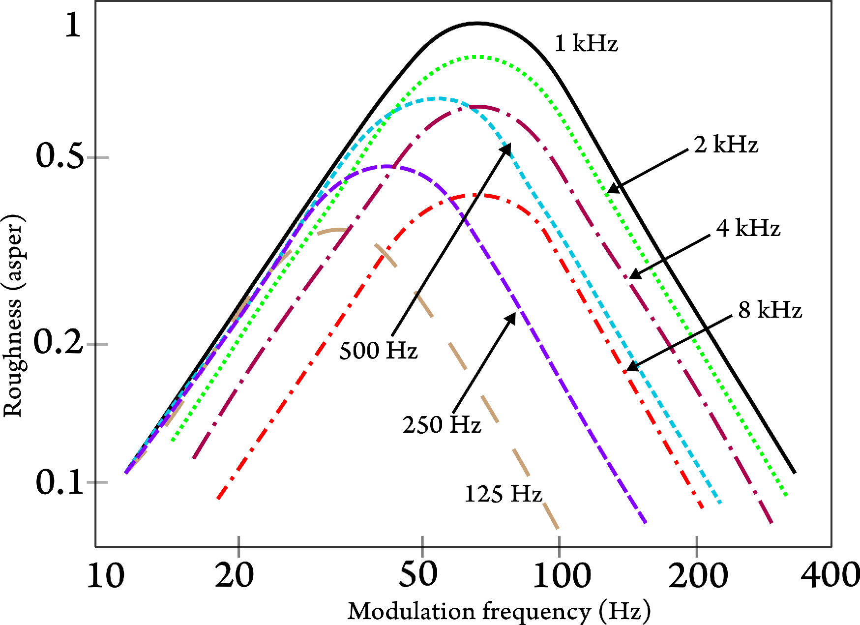
Figure 14.3: Psychoacoustic sensitivity to roughness at different carrier frequencies, as a function of the amplitude modulation frequency of the tones. The modulation depth is 1 in all cases. The figure was redrawn after Fastl and Zwicker (2007, Figure 11.2, p. 259).

A related and informal example of the effect of sampling on the TMTF can be seen in the incoherent carrier data from Viemeister (1979), who measured thresholds of modulation frequencies of up to 4000 Hz and showed that they are still audible at a -5 dB modulation depth (see Figure §13.5). However, listening to such fast modulation, it is clear that the modulation is no longer perceived as temporal at this modulation frequency, but they rather give a timbral change to the carrier, without being resolved. Thus, roughness does not apply here directly, but a similar effect happens at very high frequency, in which the temporal fluctuations are no longer audible above a certain frequency.

In summary, the empirical data presented can be used to draw a causal link between neural spikes and perceptible events. The simple consideration that has been used in all cases is whether the instantaneous sampling rate is fast enough to capture fast events in the temporal domain—a short gap, a fast pulse train, or very high modulation rates. Wheeler's “it from bit” was coined to emphasize a fundamental relation between measurable physical quantities and their informational manifestation. We borrow this expression to also include perceptual events that are carried by neural spikes.

These arguments do not preclude the existence or validity of coding of the auditory events that were described. But in the above examples, coding does not provide a parsimonious description of the measurements, because the type of errors reported (e.g., failure of detection, or drop in sensitivity) are straightforward and do not seem to merit any high-level transformations. However, hardwired aspects of coding that define the sampling patterns, such as the adaptation patterns to stimulus onset, may be considered a low-level amalgamation of sampling and coding that may be conceptually useful in all these cases.

14.7 Nonuniform undersampling

The imaging system has a finite temporal window, which must be “refreshed” in order to generate multiple images during a continuous signal, just as moving-image cameras employ shutters to periodically generate discrete images. Electronic samplers employ clocks that trigger the precisely timed samples of the analog input. Neural spikes in themselves act as irregular triggers, due to the underlying stochastic biophysical process. More centrally, the chopper cells in the cochlear nucleus might also serve the purpose of ad-hoc clocks that oscillate regularly for a brief period (§2.4). Sampling may also be the aggregate of all neural firing along the different auditory nuclei on the way downstream.

If the sampling perspective is embraced, then neural spiking represents a nonuniform-rate sampling pattern, which is conceptually different from the familiar fixed-rate sampling that was presented in §14.3. It is not the intention here to review the theory of nonuniform sampling in any depth (for example, see Marvasti, 2001), but a few key points will be highlighted, which may be intuitively understood from the vantage point of the more familiar uniform sampling.

In nonuniform sampling we generally adhere to a temporal approach that dynamically compares the instantaneous sampling rate to the Nyquist rate that is dictated by the signal spectral content. If the instantaneous frequency of the signal is above the Nyquist rate, then the signal is going to be instantaneously undersampled. The other extreme—instantaneous oversampling—is also interesting to analyze using information load considerations, rather than signal processing per se.

As real-world acoustic sources are not necessarily bandlimited, it raises a concern for aliasing that may be caused by undersampling. This is relevant here only in the context of the signal modulation spectrum bandwidth in a given auditory channel, when the modulation is not resolved in adjacent channels. High modulation frequency components that are contained in the passband have to be sampled at an appropriate rate, to avoid aliasing, unless they can be removed with an anti-aliasing filter. However, there is an interesting twist to this rule. As was first proven by Shapiro and Silverman (1960), randomizing the timing of the samples can prevent aliasing from happening in undersampling systems. Therefore, if the nonuniformity is truly random (jittering the sampling around the period does not work), then aliasing may be traded off with noise. Shapiro and Silverman (1960) also showed that if the samples are generated according to a Poisson distribution, then the reconstructed signal will be essentially alias-free¹³⁷.

Another aspect of nonuniform sampling is related to the interplay between stationary (or periodic) and nonstationary elements within continuous acoustic signals. Much of the information about the sounding objects is contained in the transient part of the signal that arrives first, before the steady-state part ensues (e.g., Kluender et al., 2003). Specifically, transient sounds can be rich in harmonics both in the carrier and in the modulation domains—depending on how they are analyzed. Therefore, it makes for an economical system design to invest more resources in sampling the transient sounds more finely than the steady-state parts of the signal that are less informative and can be sampled more slowly. This is an intuitive justification for neural adaptation in hearing, which potentially budgets the available spikes where they are most needed.

These two nonuniform sampling aspects—random sampling and denser sampling of information-rich regions of the signal—were shown to work in concert in the rhesus monkey's retina, which can be modeled as a two-dimensional spatial sampling grid (Yellott, 1983). Photoreceptor (cones) arrays on the retina are distributed in decreasing density from the highst density in the fovea, then the parafovea, the periphery, and far periphery, where the cones are sparse. One may expect that the visual image would be plagued by aliasing, if high spatial frequencies that are well-sampled by the fovea at above the Nyquist rate, are imaged by the low-density sampling periphery. However, this does not happen because the retinal sampling grid is quasi-random (not exactly Poisson-like, because of distance constraints between cones), and higher frequencies than the Nyquist rate are converted to noise in the periphery. An insightful primer about the relationship between nonuniform sampling and aliasing and how it plays out in vision was given by Resnikoff (1989, pp. 245–263).

The adaptive nature of auditory processing—its nonuniform sampling—suggests that aliasing, if observable, evokes only a fleeting sensation, as it is either replaced with internal noise, or resolved to adjacent frequency bands. In the auditory system, aliasing was conjectured to take place only during very short sequences that were tested in §E. Physiological evidence is more scant and has not invoked the terms aliasing or undersampling (with the exception of the spectral sampling model of de Cheveignè and Kawahara, 1999). A clear evidence for aliasing in auditory-nerve fiber synchronized patterns is found in Sinex and Geisler (1981, Figures 9 and 10), where instantaneous frequency was estimated by the interstimulus intervals of the spiking pattern. The fiber tracked the frequency well, but when the frequency was larger than could be sampled by the fiber, the instantaneously tracked frequencies were subharmonics of the actual instantaneous frequency—\(f/2\), \(f/3\),... \(f/6\). In other examples, occasional neural recordings of temporal modulation transfer functions seem to suggest that aliasing can be invoked artificially. See for example, Figures 2D, 5D and 5F in Kale and Heinz (2012), which show inexplicable above-cutoff-frequency responses that look like aliasing. Typically, these tuned units are taken to exhibit a band-stop (or band-reject) characteristic response (Krishna and Semple, 2000; Nelson and Carney, 2007; Carney et al., 2014), which is nevertheless difficult to distinguish from an aliased response as is seen in Figure 14.1. This ambiguity is perhaps most conspicuous in Krishna and Semple (2000), where inferior colliculus (IC) units were (over-)modulated at frequencies close to the characteristic frequency and were considered to exhibit suppressive regions caused by inhibition in the reject band, but with no clear role in sound processing (e.g., Figures 2, 4, 6, and 16).

Nonuniform sampling is presented here as an underlying reality of neural spiking, which is in large part due to its stochastic nature. However, this is not an entirely accurate representation, since the system is able to phase-lock to the carrier and synchronize to the envelope. We modeled phase locking earlier as a result of a dedicated phase-locked loop (PLL) module in the cochlea (§9). One of the most important usages of PLLs in communication circuits is synchronization of the internal signal to the external one, which was produced remotely using a local oscillator, which works as a clock. The PLL therefore obviates the need for a local clock at the receiver, as long as ad-hoc samples can be generated that are synchronized to the signal¹³⁸. If the PLL is out of lock, then the randomness of its samples is expected to increase.

14.8 The effect of sampling on the modulation transfer function

Having clarified some of the main features of the sampling auditory system, we would like to account for the discrepancy in the bandwidth of the predicted and the empirical TMTFs we analyzed in §13.4. From the analysis of the various auditory TMTFs, it appears that the cutoff frequency predictions made using the ideal ATF (Figure §13.2) grossly overestimate the behavioral coherent response values compared to findings from literature (Figure §13.4). The same is true for the incoherent TMTF, although the general property of a smaller incoherent than coherent TMTF bandwidth was predicted correctly. How can this discrepancy be explained, given that the very same parameters have been used fairly successfully to predict the behavioral curvature and temporal aperture data in §12.4?

One possible explanation for the MTF and TMTF discrepancy may be related to the fact that some auditory brainstem units are better described by bandpass rather than by low-pass modulation response. For example, in the guinea-pig's ventral cochlear nucleus (VCN), several tuned unit types (primary, sustained choppers, and onset chopper cells) have characteristic responses to sinusoidal amplitude modulation that are less low-pass and more bandpass in their response, as they display a clear peak at their best modulation frequency (e.g., Sayles et al., 2013). At full modulation depth most units appear low-pass, but become bandpass with lower modulation depth values—mainly the chopper units that are most sensitive to AM. However, the high-frequency response of these bandpass units overlaps that of the low-pass units, so even if the characteristic filtering of these cells is relatively dominant in the VCN overall response (and eventual perception), it still does not explain the complete lack of sensitivity to high frequencies in behavioral tests. Rather, it appears to be shaping the low-frequency irregularities that are sometimes observed in empirical data (Figure §13.3), which were also discussed in the context of narrowband responses (§13.4.5).

An alternative explanation for the discrepancy in the MTF prediction is due to sampling limitations. There are at least three known causes for MTF degradations and bandwidth reduction in optics that are caused by finite spatial sampling of the image (Wittenstein et al., 1982; Park et al., 1984; de Luca and Cardone, 1991; Boreman, 2001; pp. 35–50). First, the assumption of time-invariance¹³⁹ is generally not true for a sampler that has a finite sampling frequency \(f_s\). This means that small delays of the object—of the order of one sampling period—can heighten the sensitivity to slightly different features that are captured by its finite-sized samples. This is compounded by the second cause, which is that real-world objects are generally not bandlimited, so that arbitrary inputs that contain modulation frequencies that are higher than its instantaneous Nyquist rate \(f_m>f_s/2\) can be aliased. The third cause is the finite footprint of the optical detector, which in our case is equivalent to sampling that is not impulse-like (§14.4). In optical detectors, the basic unit of detection is at minimum one pixel, which assumes a constant intensity that effectively produces flat-top sampling (§14.4.3). While we do not expect it to be exactly the case in hearing, we know that the finite size and response of each sample has an effect on the image. In spatial optics, the compounded effect of sampling on MTF is captured by the sampling MTF following the detector, which is located at a distance behind the lens. In the hearing system, the first sampling location is right after the lens, before the neural group-delay dispersion. We will nevertheless consider the effect to be qualitatively the same as in spatial imaging.

The main difference between the psychoacoustic phase curvature (§12.4) and the MTF predictions is that the former was based on the time-domain imaging transform and the latter on frequency-domain transfer functions. The time-domain model we developed for the phase curvature data relied on a single image of the stimulus—a snapshot of a pulse—which contains all the information necessary for solving that problem. Using frequency-domain methods for long stimuli, though, we are required to integrate over many pulses that are sampled across fibers over a long time. For this to work, sampling has to be perfect, so that the sampling MTF can be exactly equal to the MTF, over several synapses—each of which resamples the previously sampled MTF. As perfect sampling is unlikely to take place, we can expect the signal to be gradually undersampled by the time it reaches the auditory retina at the IC.

The role of undersampling in the received TMTF is supported by animal data—as long as it is reinterpreted according to a sampling framework. On the whole, TMTFs that are measured along the auditory pathways, between the auditory nerve and the midrain and auditory cortex, gradually become less sensitive to high modulation frequencies and rate coding becomes more prevalent beyond the IC (for a comprehensive summary, see Joris et al., 2004, Figure 9). For example, despite broadened cochlear filters due to noise-induced hearing loss, broadening had no effect on the modulation bandwidth in the auditory nerve of chinchillas. It was suggested that the TMTF is constrained by non-cochlear factors, such as neural adaptation and refractoriness (Kale and Heinz, 2010; Kale and Heinz, 2012; Kale et al., 2014; See §17.3.4 for further discussion). Incidentally, it fits our earlier conclusion that the aperture stop of the system is determined by the neural transduction and not by the cochlear filters.

In another recent study, data from the Mongolian gerbil, which were based on realistic stimuli from its natural environment, showed that some parts of the stimulus are postsynaptically inhibited between the auditory nerve and the spherical bushy cells in the anteroventral cochlear nucleus (AVCN) (Keine et al., 2017). Sampling considerations can suggest that many samples are lost between the auditory nerve and the AVCN, which effectively results in a substantial drop in the transmitted information and, hence, in a drop in the effective sampling rate. Notably, though, the recorded rate in these cells was comparable to their spontaneous activity rate. Additionally, the reduction in the instantaneous firing rate resulted in a complementary increase in the temporal precision of the samples. Similar results were reported by Dehmel et al. (2010) and Kuenzel et al. (2011).

The decrease in sampling rates in the gerbil is reminiscent of the starling data we reviewed earlier by Klump and Gleich (1991) and Gleich and Klump (1995), who found that the behavioral modulation bandwidth was about half of the physiological one (§13.4.4). Our prediction was only 7% higher than the physiological value that was recorded from the auditory nerve of the starling. We can try to supplement these findings by estimating how critical the effect of undersampling is, by comparing the predictions we obtained for the perfectly sampled MTF in humans to the fastest known synchronized modulation rates that were reported in physiological studies. As was reviewed in §13.4.3, the highest modulation frequencies that were measured in the auditory nerve of any species are from the cat and are in the range of 1500–2500 Hz for carriers of 10–30 kHz (Rhode and Greenberg, 1994; Figure 13). Therefore, our predictions still overestimate the frequency cutoff of the MTFs, as it we see up to 3000 Hz modulation cutoff at 10 kHz (Figure §13.2)¹⁴⁰.

Our predictions of human compared to both cat and starling maximum cutoff measurements suggest that in any case they are overestimated. Accounting for undersampling definitely appears to contribute to the discrepancy, especially if it begins early on—as soon as the mechanical signal is transduced. But these results are also confounded by the uncertainty we have about the dispersion parameters, especially at high-frequency carriers, which likely skew the results. Furthermore, the simple modeling offered by the MTF does not take into account the evident physiological limitation for synchronizing to high modulation frequencies, perhaps due to refractoriness.

A final mechanism for degradation of the coherent TMTF should be mentioned, which is not independent from the undersampling mechanism. Both undersampling and nonuniformity effectively contribute to the decoherence of the coherently detected signal. This is encountered in the auditory nerve, but we also mentioned examples for AVCN units that retain their low modulation frequency precision in spite of undersampling, although these observations did not apply for all cells (Dehmel et al., 2010; Kuenzel et al., 2011; Keine et al., 2017). This may mean that other subpopulations of cells in AVCN and perhaps in other nuclei may not conserve the coherence of the incoming signal, which depends on the phase-locking precision, on top of the MTF bandwidth. It is therefore possible that as the signal becomes partially coherent, its MTF becomes closer to that of the incoherent MTF, which has a more limited bandwidth.

14.9 Discussion

The role of sampling in auditory processing was analyzed with special attention given to the type of sampling window, the effect of nonuniform sampling, and potential aliasing. It was then used to account for the bandwidth narrowing in the measured TMTF compared to the predicted MTF, which was based on perfectly sampled frequency-domain transforms. We identified the auditory nerve as the primary site of sampling, but noted that repeated resamping throughout the brain is a likely source of further degradation in the perceived MTF.

The sample, which is the sound image of a pulse, may represent the minimal unit of auditory perception that can be experimentally observed both physiologically and psychoacoustically. We produced some evidence to attest to that the image might contain more information than an optical pixel, which is defined by its fixed place and intensity reading. Further work will have to be done to find out what the most appropriate relationship is between the image and the sample, or how much information is contained in a single spike. Also, given that information is pooled over populations of fibers in every channel and usually over several channels, then the perceptual significance of a single image-sample as the atom of hearing (similar to Gabor's logon, Gabor, 1946) has to be clarified.

Neural sampling of continuous signals poses a few conceptual challenges that have been either neglected or treated only in passing in various hearing models. We would like to flag some of these challenges in advance, as they can guide the discussion that follows. These challenges are not going to be necessarily resolved in this work, though, as our main goal is to see how sampling implicate temporal imaging.

Embracing the notion of neural sampling comes close to suggesting that the auditory brain operates discretely and not continuously. This is a highly contentious topic in neuroscience that has been avoided in auditory research almost completely (but see VanRullen et al., 2014). Although the experience of our auditory perception (and other modalities too) feels continuous and not discrete, there are more than a handful of results that indicate that it is a finely sampled sequence of discrete images, which only appear continuous. If the IC is assigned the role of the auditory retina (§11.7), then beyond it the discrete/continuous representation problem is reduced to that of visual processing downstream from the retina, as long as thalamic and cortical processing is directly comparable between the two modalities (see §1.5.2). Additional discussion is found in §E.3.

A major requirement in sampling, which was implicit throughout the chapter, is that it should lead to reconstruction of the signal at the output. However, we have no access to the notion of signal reconstruction in perception, so we cannot estimate what the relevance of this mathematical concept is to the brain. Nevertheless, it has been insightful to discuss sampling as a goal-oriented process, which can be evaluated by comparing it to an ideal process from which the signal can be faithfully recovered.

We discussed the implications of nonuniform sampling with emphasis on undersampled inputs that cause aliasing, but we did not touch the concept of oversampling. In theory, oversampling provides a fail-proof solution to distortion from aliasing, so it may appear like a good strategy. However, it is also wasteful in that it produces larger quantities of data than may be needed and can load the system informationally, cognitively, and also in terms of the incurred energy costs. Therefore, it can be argued that unnecessary information is readily discarded in hearing, using only a minimal number of samples that are needed to just represent the stimulus correctly and maintain a sense of continuity (Weisser, 2019). See also §E.2.3.

Footnotes

131. Dithering is smoothing of sampling fluctuations, which are caused by the minimum quantization level (its finite resolution), through the addition of random low-level noise.

132. The existence of an actual reconstruction operation will remain, at this stage, completely hypothetical insofar as it pertains to auditory perception.

133. Wheeler (1990).

134. Higher onset discharge rates were recorded in the auditory nerve of the chinchilla of about 2700 spikes per second (!) (Ruggero, 1992; Figure 2.6).

135. Note that in an attempt to model psychoacoustical forward masking patterns using either neural adaptation or temporal integration models, the former was disfavored and produced somehow less good fit than the latter (Oxenham, 2001). In that analysis Oxenham suggested that neural adaptation effects may be altogether ignored at the level of the periphery. For a higher-level review of auditory adaptation, see Willmore and King (2023).

136. The 8 kHz frequency band can be made to work with the sharper filters reported in Oxenham and Shera (2003) (see §11.6.3), which produce about half the bandwidth at this frequency (212 Hz), but predicts better spectral resolution at 250 Hz and less roughness. Figure 14.3 shows no roughness at 250 Hz. However, this explanation does not work for lower carrier frequencies, which have a smaller absolute bandwidth, but high maximum modulation frequency for roughness sensation. For example, at 2 kHz carrier, the same calculation produces a limit of 75 Hz, while the data show that some roughness exists at least up to 300 Hz.

137. A modern signal-processing approach to undersampling that is called compressed sensing is based on different mathematical principles than those of Shapiro and Silverman (1960). Compressed sensing has been successfully employed in signal processing applications to beat the aliasing limit imposed by the Nyquist rate (Candes et al., 2004). It makes use of a known but general functional basis (e.g., wavelets) that is taken as background information, which reduces the need for many samples to be generated with regular clocking. Neural correlates of this techniques have been theorized (Ganguli and Sompolinsky, 2012), but none were studied in the auditory system to date, although the earlier model by Benedetto and Teolis (1993) and Benedetto and Scott (2001) is also based on nonuniform sampling with a wavelet basis and might be conceptually related. Compressed sensing has found much use in image compression (Patel and Chellappa, 2013), for example, but will not be dealt with here, as it is not clear that it reflects the physiological auditory signal processing.

138. Clocks have appeared rather rarely in auditory models, although usually only with short-term regularity and without a clear physiological correlate (e.g., Whitfield, 1970; Suga and Schlegel, 1973; Yang et al., 2018).

139. Shift-invariance in spatial imaging.

140. Unfortunately, the dispersion parameters above 10 kHz are extrapolated and are very unstable and therefore could not be reliably used to estimate higher MTF cutoff frequencies.

References

Adrian, Edgar D and Zotterman, Yngve. The impulses produced by sensory nerve-endings: Part II. The response of a single end-organ. The Journal of Physiology, 61 (2): 151–171, 1926.

Benedetto, John J and Teolis, Anthony. A wavelet auditory model and data compression. Applied and Computational Harmonic Analysis, 1 (1): 3–28, 1993.

Benedetto, JJ and Scott, S. Frames, irregular sampling, and a wavelet auditory model. In Marvasti, Farokh, editor, Nonuniform Sampling: Theory and Practice, pages 585–617. Springer Science+Business Media, LLC, New York, NY, 2001.

Bialek, William. Physical limits to sensation and perception. Annual Review of Biophysics and Biophysical Chemistry, 16 (1): 455–478, 1987.

Boreman, Glenn D. Modulation transfer function in optical and electro-optical systems, volume TT52. SPIE Press – The International Society for Optical Engineering, Bellingham, WA, 2001.

Brette, Romain. Is coding a relevant metaphor for the brain? Behavioral and Brain Sciences, 42: 1–58, 2019.

Buchfellner, Elisabeth, Leppelsack, Hans-Joachim, Klump, Georg M, and Häusler, Udo. Gap detection in the starling (sturnus vulgaris). Journal of Comparative Physiology A, 164 (4): 539–549, 1989.

Candes, Emmanuel, Romberg, Justin, and Tao, Terence. Robust uncertainty principles: Exact signal reconstruction from highly incomplete frequency information. arXiv preprint math/0409186, 2004.

Carney, Laurel H, Zilany, Muhammad SA, Huang, Nicholas J, Abrams, Kristina S, and Idrobo, Fabio. Suboptimal use of neural information in a mammalian auditory system. Journal of Neuroscience, 34 (4): 1306–1313, 2014.

de Cheveigné, Alain. Pitch perception models. In Plack, Christopher J, Oxenham, Andrew J, Fay, Richard R., and Popper, Arthur N., editors, Pitch. Springer, 2005.

Couch II, Leon W. Digital and Analog Communication Systems. Pearson Education Inc., Upper Saddle River, NJ, 8th edition, 2013.

Dehmel, Susanne, Kopp-Scheinpflug, Cornelia, Weick, Michael, Dörrscheidt, Gerd J, and Rübsamen, Rudolf. Transmission of phase-coupling accuracy from the auditory nerve to spherical bushy cells in the mongolian gerbil. Hearing Research, 268 (1-2): 234–249, 2010.

Doughty, JM and Garner, WR. Pitch characteristics of short tones. I. Two kinds of pitch threshold. Journal of Experimental Psychology, 37 (4): 351, 1947.

Fastl, Hugo and Zwicker, Eberhard. Psychoacoustics: Facts and Models. Springer Science & Business Media, 3rd edition, 2007.

Gabor, Dennis. Theory of communication. Part 1: The analysis of information. Journal of the Institution of Electrical Engineers-Part III: Radio and Communication Engineering, 93 (26): 429–457, 1946.

Galambos, Robert and Davis, Hallowell. The response of single auditory-nerve fibers to acoustic stimulation. Journal of Neurophysiology, 6 (1): 39–57, 1943.

Ganguli, Surya and Sompolinsky, Haim. Compressed sensing, sparsity, and dimensionality in neuronal information processing and data analysis. Annual review of Neuroscience, 35: 485–508, 2012.

Garson, Justin. The birth of information in the brain: Edgar Adrian and the vacuum tube. Science in Context, 28 (1): 31–52, 2015.

Glasberg, Brian R and Moore, Brian CJ. Derivation of auditory filter shapes from notched-noise data. Hearing Research, 47 (1-2): 103–138, 1990.

Gleich, Otto and Klump, Georg M. Temporal modulation transfer functions in the European Starling (Sturnus vulgaris): II. Responses of auditory-nerve fibres. Hearing Research, 82 (1): 81–92, 1995.

Heil, Peter. Coding of temporal onset envelope in the auditory system. Speech Communication, 41 (1): 123–134, 2003.

Heil, Peter and Irvine, Dexter RF. First-spike timing of auditory-nerve fibers and comparison with auditory cortex. Journal of neurophysiology, 78 (5): 2438–2454, 1997.

Joris, PX, Schreiner, CE, and Rees, A. Neural processing of amplitude-modulated sounds. Physiological Reviews, 84 (2): 541–577, 2004.

Kale, Sushrut and Heinz, Michael G. Envelope coding in auditory nerve fibers following noise-induced hearing loss. Journal of the Association for Research in Otolaryngology, 11 (4): 657–673, 2010.

Kale, Sushrut and Heinz, Michael G. Temporal modulation transfer functions measured from auditory-nerve responses following sensorineural hearing loss. Hearing Research, 286 (1-2): 64–75, 2012.

Kale, Sushrut, Micheyl, Christophe, and Heinz, Michael G. Implications of within-fiber temporal coding for perceptual studies of f0 discrimination and discrimination of harmonic and inharmonic tone complexes. Journal of the Association for Research in Otolaryngology, 15 (3): 465–482, 2014.

Keine, Christian, Rübsamen, Rudolf, and Englitz, Bernhard. Signal integration at spherical bushy cells enhances representation of temporal structure but limits its range. eLife, 6: e29639, 2017.

Kiang, Nelson Yuan-Sheng, Watanabe, Takeshi, Thomas, Eleanor C., and Clark, Louise F. Discharge patterns of single fibers in the cat's auditory nerve. In Research Monograph No. 35. The M.I.T. Press, Cambridge, MA, 1965.

Kluender, Keith R, Coady, Jeffry A, and Kiefte, Michael. Sensitivity to change in perception of speech. Speech Communication, 41 (1): 59–69, 2003.

Klump, Georg M and Maier, Elke H. Gap detection in the starling (Sturnus vulgaris). Journal of Comparative Physiology A, 164 (4): 531–538, 1989.

Klump, Georg M and Gleich, Otto. Gap detection in the European starling (Sturnus vulgaris). Journal of Comparative Physiology A, 168 (4): 469–476, 1991.

Krishna, B Suresh and Semple, Malcolm N. Auditory temporal processing: Responses to sinusoidally amplitude-modulated tones in the inferior colliculus. Journal of Neurophysiology, 84 (1): 255–273, 2000.

Kuenzel, Thomas, Borst, J Gerard G, and van der Heijden, Marcel. Factors controlling the input–output relationship of spherical bushy cells in the gerbil cochlear nucleus. Journal of Neuroscience, 31 (11): 4260–4273, 2011.

Landauer, Rolf. The physical nature of information. Physics Letters A, 217 (4-5): 188–193, 1996.

Lewis, Edwin R and Henry, Kenneth R. Nonlinear effects of noise on phase-locked cochlear-nerve responses to sinusoidal stimuli. Hearing Research, 92 (1-2): 1–16, 1995.

Lyon, Richard F. Human and Machine Hearing. Cambridge University Press, 2018. Author's corrected manuscript.

Marvasti, Farokh. Nonuniform Sampling – Theory and Practice. Springer Science+Business Media, LLC, New York, NY, 2001.

Nelson, Paul C and Carney, Laurel H. Neural rate and timing cues for detection and discrimination of amplitude-modulated tones in the awake rabbit inferior colliculus. Journal of Neurophysiology, 97 (1): 522–539, 2007.

Oxenham, Andrew J. Forward masking: Adaptation or integration? The Journal of the Acoustical Society of America, 109 (2): 732–741, 2001.

Oxenham, Andrew J and Kreft, Heather A. Speech perception in tones and noise via cochlear implants reveals influence of spectral resolution on temporal processing. Trends in Hearing, 18: 1–14, 2014.

Oxenham, Andrew J and Shera, Christopher A. Estimates of human cochlear tuning at low levels using forward and simultaneous masking. Journal of the Association for Research in Otolaryngology, 4 (4): 541–554, 2003.

Park, Stephen K, Schowengerdt, Robert, and Kaczynski, Mary-Anne. Modulation-transfer-function analysis for sampled image systems. Applied Optics, 23 (15): 2572–2582, 1984.

Patel, Vishal M and Chellappa, Rama. Sparse representations and compressive sensing for imaging and vision. Springer Science & Business Media, 2013.

Patterson, Roy D, Robinson, K, Holdsworth, J, McKeown, D, Zhang, C, and Allerhand, M. Complex sounds and auditory images. In Cazals, Y., Horner, K., and Demany, L., editors, Auditory Physiology and Perception, volume 83, pages 429–446. Pergamon Press, Oxford, United Kingdom, 1992.

Pelgrom, Marcel JM. Analog-to-digital conversion. In Analog-to-Digital Conversion. Springer Science+Business Media B.V., 2010.

Perkel, Donald H and Bullock, Theodore H. Neural coding. Neurosciences Research Program Bulletin, 6 (3): 221–348, 1968.

Poeppel, David. The analysis of speech in different temporal integration windows: Cerebral lateralization as 'asymmetric sampling in time'. Speech Communication, 41 (1): 245–255, 2003.

Lopez-Poveda, Enrique A and Eustaquio-Martin, Almudena. On the controversy about the sharpness of human cochlear tuning. Journal of the Association for Research in Otolaryngology, 14 (5): 673–686, 2013b.

Lopez-Poveda, Enrique A. Why do i hear but not understand? stochastic undersampling as a model of degraded neural encoding of speech. Frontiers in Neuroscience, 8: 348, 2014.

Resnikoff, Howard L. The Illusion of Reality. Springer-Verlag New York Inc., 1989.

Rhode, William S and Greenberg, Steven. Encoding of amplitude modulation in the cochlear nucleus of the cat. Journal of Neurophysiology, 71 (5): 1797–1825, 1994.

Ruggero, Mario A. Physiology and coding of sound in the auditory nerve. In Popper, Arthur N. and Fay, Richard R., editors, The Mammalian Auditory Pathway: Neurophysiology, volume 2, pages 34–93. Springer-Verlag New York, Inc., 1992.

Sanderson, Mark I, Neretti, Nicola, Intrator, Nathan, and Simmons, James A. Evaluation of an auditory model for echo delay accuracy in wideband biosonar. The Journal of the Acoustical Society of America, 114 (3): 1648–1659, 2003.

Sayles, Mark, Füllgrabe, Christian, and Winter, Ian M. Neurometric amplitude-modulation detection threshold in the guinea-pig ventral cochlear nucleus. The Journal of Physiology, 591 (13): 3401–3419, 2013.

Shannon, Claude E. A mathematical theory of communication. The Bell System Technical Journal, 27 (3): 379–423, 623–656, 1948.

Shannon, Claude E. The bandwagon. IRE Transactions on Information Theory, 2 (1): 3, 1956.

Shapiro, Harold S and Silverman, Richard A. Alias-free sampling of random noise. Journal of the Society for Industrial and Applied Mathematics, 8 (2): 225–248, 1960.

Simmons, James A, Ferragamo, Michael, Moss, Cynthia F, Stevenson, Scott B, and Altes, Richard A. Discrimination of jittered sonar echoes by the echolocating bat, eptesicus fuscus: The shape of target images in echolocation. Journal of Comparative Physiology A, 167 (5): 589–616, 1990.

Simmons, James A, Saillant, Prestor A, Ferragamo, Michael J, Haresign, Tim, Dear, Steven P, Fritz, Jonathan, and McMullen, Teresa A. Auditory computations for biosonar target imaging in bats. In Hawkings, Harold L, McMullen, Teresa A, Popper, Arnold N, and Fay, Richard R, editors, Auditory Computation, pages 401–468. Springer-Verlag New York Inc., New York, NY, 1996.

Sinex, Donal G and Geisler, C Daniel. Auditory-nerve fiber responses to frequency-modulated tones. Hearing Research, 4 (2): 127–148, 1981.

Suga, Nobuo and Schlegel, Peter. Coding and processing in the auditory systems of fm-signal-producing bats. The Journal of the Acoustical Society of America, 54 (1): 174–190, 1973.

Unser, Michael. Sampling—50 years after Shannon. Proceedings of the IEEE, 88 (4): 569–587, 2000.

VanRullen, Rufin, Zoefel, Benedikt, and Ilhan, Barkin. On the cyclic nature of perception in vision versus audition. Philosophical Transactions of the Royal Society B: Biological Sciences, 369 (1641): 20130214, 2014.

Viemeister, Neal F. Temporal modulation transfer functions based upon modulation thresholds. The Journal of the Acoustical Society of America, 66 (5): 1364–1380, 1979.

Viemeister, Neal F and Wakefield, Gregory H. Temporal integration and multiple looks. The Journal of the Acoustical Society of America, 90 (2): 858–865, 1991.

Warchol, Mark E and Dallos, Peter. Neural coding in the chick cochlear nucleus. Journal of Comparative Physiology A, 166 (5): 721–734, 1990.

Weisser, Adam. Auditory information loss in real-world listening environments. arXiv preprint arXiv:1902.07509, 2019.

Westerman, Larry A and Smith, Robert L. Rapid and short-term adaptation in auditory nerve responses. Hearing Research, 15 (3): 249–260, 1984.

Wever, Ernest Glen and Bray, Charles William. Present possibilities for auditory theory. The Psychological Review, 37 (5): 365, 1930b.

Wever, Ernest Glen. Theory of Hearing. John Wiley & Sons New York, Chapman & Hall Limited, London, 1949.

Wheeler, John A. Information, physics, quantum: The search for links. In Zurek, Wojciech H., editor, Complexity, Entropy, and the Physics of Information. Addison-Wesley, Reading, MA, 1990.

Whitfield, I. C. Central nervous processing in relation to spatio-temporal discrimination of auditory patterns. In Plomp, R. and Smoorenburg, G. F., editors, Frequency Analysis and Periodicity Detection in Hearing, pages 136–152. A. W. Sijthoff, Leiden, 1970.

Willmore, Ben DB and King, Andrew J. Adaptation in auditory processing. Physiological Reviews, 103 (2): 1025–1058, 2023.

Wittenstein, W, Fontanella, JC, Newbery, AR, and Baars, J. The definition of the OTF and the measurement of aliasing for sampled imaging systems. Optica Acta: International Journal of Optics, 29 (1): 41–50, 1982.

Yamada, Walter Masami and Lewis, Edwin R. Predicting the temporal responses of non-phase-locking bullfrog auditory units to complex acoustic waveforms. Hearing Research, 130 (1-2): 155–170, 1999.

Yang, Xiaowei, Wang, Kuansan, and Shamma, Shihab A. Auditory representations of acoustic signals. IEEE Transactions on Information Theory, 38 (2): 824–839, 1992.

Yang, Sunggu, Chung, Jaeyong, Jin, Sung Hun, Bao, Shaowen, and Yang, Sungchil. A circuit mechanism of time-to-space conversion for perception. Hearing Research, 2018.

Yellott, John I. Spectral consequences of photoreceptor sampling in the rhesus retina. Science, 221 (4608): 382–385, 1983.

de Cheveignè, Alain and Kawahara, Hideki. Missing-data model of vowel identification. The Journal of the Acoustical Society of America, 105 (6): 3497–3508, 1999.

de Luca, Luigi and Cardone, Gennaro. Modulation transfer function cascade model for a sampled IR imaging system. Applied optics, 30 (13): 1659–1664, 1991.