Chapter 11

Estimating the auditory imaging parameters

11.1 Introduction

All physical systems are dispersive to a certain extent (Brillouin, 1960) and various dispersive phenomena have been reviewed in §3 to illustrate it in acoustical systems. Therefore, it should not be surprising to encounter dispersive effects in the hearing organs as well. While it has been commonly accepted that the cochlea is dispersive, other parts of the system are not explicitly considered to be so. Most importantly, second-order dispersive effects—group velocity (or group delay) dispersion—are even more rarely considered and are not given any special significance, and are often assumed to have negligible effects on hearing.

Based on available findings from literature, in this chapter we attempt to estimate the human group-velocity dispersion along the auditory system—the outer ear, middle ear, inner ear, and brainstem. As will be seen, dispersion is always frequency-dependent, which results in non-negligible group-delay dispersion. Conveniently, consecutive dispersive paths are additive (being phase arguments) and may be factored into single parameters (§B.3). The main segments that will be identified are the cochlear dispersion up to the organ of Corti, the time lens of the organ of Corti, and the neural dispersion from the inner hair cells (IHCs) to the inferior colliculus (IC). These segments will inform the subsequent temporal imaging analysis. See Figure 11.1 for the rough segmentation of the system considered here.

Throughout this chapter, the effects of bone conduction hearing are neglected. While it is well-known that the outer and middle ear stages of the ear may be bypassed through bone conduction (Békésy, 1948), the effect is not dominant in normal conditions, with the exception of some sea mammals (§2.5.1) and in listeners with severe conductive losses that must rely on bone conduction for hearing.

All data from published figures in this chapter and throughout this work were digitized using WebPlotDigitizer⁹⁷ and analyzed in Matlab (the Mathworks Inc.).

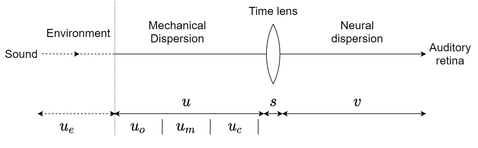
Figure 11.1: The rough division of the auditory system to dispersive elements. The mechanical parts of the ear are combined into one group-delay-dispersive parameter, \(u\), with contributions from the outer ear \(u_o\), the middle ear \(u_m\), and the cochlea \(u_c\). The time lens with curvature \(s\) is hypothesized to be mechanically incorporated in the organ of Corti and neurally controlled (accommodated; §16.4.2). The neural group-delay dispersion \(v\) begins as late as the auditory nerve, but may also comprise the inner hair cells and the passive transmission in the organ of Corti. The external group-delay dispersion in the environment \(u_e\) is not considered directly in the analysis, but is assumed to be relatively low compared to \(u\) in normal atmospheric conditions and over short distances.

11.2 The outer ear

The outer ear is the first organ to receive the information carried by acoustic waves in air or in water, neglecting bone conduction. By the time the sound reaches the outer ears, it has accumulated a degree of dispersion that is proportional to the distance it has traversed in the medium, often including additional reflections. As was shown in §3.4.2, the atmospheric dispersion is generally negligible over small distances, but it may be susceptible to unpredictable weather conditions and to other environmental factors, which likely affect the group-velocity dispersion as well. Another uncertainty is the combination of acoustic modes that carry the information at the point of entrance to the ear. As was noted in the previous chapter, the temporal imaging equations are well-defined only for plane waves, where higher-order modes are absent. In this light, the outer ear seems to play an important role, as it imposes a unimodal, plane-wave-only, transmission over a significant portion of the audio spectrum.

11.2.1 The waveguide approximation

To a first approximation, the outer ear is an acoustic waveguide, shaped as a pipe that is closed in one end. Wave propagation in pipes is typically analyzed in terms of normal modes, which can be spatially distributed in different ways, according to the geometry of the pipe (for illustration, see Fletcher and Rossing, 1998; p. 193). Ideal waveguides act as transmission lines and allow acoustic energy to be carried only in the plane wave mode, as long as the wavelength of the sound is much longer than the diameter of the tube, \(\lambda \gg D\) (Morse and Ingard, 1968; pp. 471–472). Higher modes do not exist below a certain cutoff frequency, where their phase velocity is infinite. Above this cutoff, the phase velocity decreases quickly. If the tube walls are yielding—if they are not entirely rigid, but have a finite compliance—then they locally react to the pressure gradient of the plane wave⁹⁸ (Morse and Ingard, 1968; pp. 475-477). This results in frequency-dependent phase velocity as a function of the wall material and resonances for the particular pipe geometry. It means that the low-frequency waves travel faster than the high-frequency ones—dispersion. When the one-dimensional plane-wave approximation breaks down, additional modes appear as some of the sound waves begin to propagate along the waveguide circumference rather than in its center (Morse and Ingard, 1968; pp. 688–689). Applying the simplistic rigid-wall waveguide limit to the human ear canal geometry, and using a typical ear canal diameter of 0.7 cm (Goode et al., 1977; cited in Rabbitt and Holmes, 1988), or from cross-sectional data 0.75 cm (Rosowski, 1994), indicates a strict plane-wave propagation of up to about 24.5 kHz of sound in air, at normal room temperature, for an open-ended waveguide. Keefe et al. (1993) reported growing diameters with age with adult diameter of 1.04 cm, corresponding to a 16.5 kHz cutoff. However, these cutoff values are unrealistic, as is shown next.

11.2.2 Higher-order modes

In a real outer ear, strict plane-wave propagation breaks down at much lower frequencies than predicted by the waveguide approximation due to the complex geometry of the ear canal. When sound arrives from the environment to the outer ear, it is scattered by the concha, which creates various non-planar modes, mainly at high frequencies (Rabbitt and Holmes, 1988; Rabbitt and Friedrich, 1991). However, these modes quickly vanish once inside the ear canal, as the plane-wave mode becomes dominant within a few millimeters, even at high frequencies (Rabbitt and Friedrich, 1991; Hudde and Schmidt, 2009). Three-dimensional simulations of sound waves in the bent human ear canal showed that the ear canal has additional non-planar modes that are trapped around its bends, but these modes also vanish very quickly and do not interfere with the plane wave propagation (Hudde and Schmidt, 2009).

Analytic approximation to the solution of the wave equation of the ear canal found that higher vibrational modes start to be present from about 4 kHz (Rabbitt and Holmes, 1988). These modes are formed by the eardrum (the pars tensa) itself due to its elasticity and geometry that is detached from the ear canal walls. With increasing frequency the eardrum modes tend to extend spatially to the interior of the ear canal, and these modes are reflected back to the canal and interact with its trapped modes. This may explain an effect of probe microphone response variance as a function of distance from the eardrum above 4 kHz (Caldwell et al., 2006). Holographic measurements of the eardrum revealed modes above 1 kHz, which grow in dominance at higher frequencies (Cheng et al., 2013). The effect extends even to the middle ear, as impedance measurements of the cat's middle ear were best modeled by including standing waves of the eardrum above 3 kHz, which produced a measurable transmission delay (Puria and Allen, 1998). Therefore, the dominant non-planar, and thus dispersive, mechanism in the ear canal is not a result of yielding walls, but rather of the tube coupling to the compliant, oddly shaped eardrum, which is itself yielding.

All together, the pressure wave that arrives to the middle ear is the sum of all the modes that make it to the eardrum. So, at frequencies below 5 kHz the relative coupling of the non-planar higher-order modes in the ear canal to the movement of the eardrum is about 10% for children and close to 30% for adults, and about 25% at 4 kHz (Rabbitt and Holmes, 1988). Hudde and Schmidt (2009) found that the eardrum minimally disturbs the plane-wave mode below 4 kHz, despite its compliance and middle ear resonances above 1 kHz.

One question remains unanswered regarding the high-frequency domain above 4 kHz, where non-planar modes carry more energy: is there any dispersion distortion (§10.4) that affects the information entering the middle ear? The topic has not been considered at all in the acoustic literature. However, indirect data from the cat suggest that dispersion distortion may be a real problem. Probe microphone measurements in the cat's ear canal show that above 10 kHz the variation of pressure over the eardrum surface makes it impossible to have one reference or mean level that is confidently conducted to the middle ear, due to anomalous high-frequency response (Khanna and Stinson, 1985). In another perspective, it was demonstrated through simulations that the multitude of normal modes at high frequencies is advantageous in terms of energy distribution, and hence, power transmission to the middle ear (Fay et al., 2006).

In conclusion, treating the ear canal as one-dimensional plane wave conduit is a justified assumption below 4 kHz in humans, in line with the dispersion equation assumptions. At higher frequencies, the validity of this assumption is expected to progressively drop, but to an unknown degree. The specific cutoff is most certaintly different in other animals with different ear geometries.

11.2.3 The group-velocity dispersion of the outer ear

The group-velocity dispersion will be estimated using published phase or group delay data.

In measuring the phase response of the outer ear, the results may be susceptible to large errors due to small variations in measurement positions at frequencies above 4 kHz, the small dimensions involved, the resonances of the ear canal, finite dimensions of the microphone, and access to the eardrum (Brass and Locke, 1997; Caldwell et al., 2006). Figure 11.2 reproduces ear-canal phase and group delay data compiled from various studies, which employed different techniques to obtain phase measurements, all at slightly different measurement positions. Ear canal phase data was obtained from three subjects by Mehrgardt and Mellert (1977) for a free-field source by subtracting the response of a free-field microphone positioned at the ear canal entrance from the response of a probe microphone near the eardrum, 20 cm from the entrance (top left). Data from Rasetshwane and Neely (2011) (top right) are full-spectrum reflectance group delay measurements averaged from 24 individual subjects. Similar data from two additional subjects were reported by Keefe et al. (1993) for a narrower spectrum (bottom left). These measurements were obtained by sealing the ear canal, and flush-mounting a miniature sound source on the seal, while a probe microphone was positioned right outside the eardrum. The group delay of these measurements accounts for the round trip of the pressure wave, so they were divided by two (Voss et al., 2000). Finally, direct measurements of the group delay in the ear canal of 11 subjects were also provided by Blauert (1997), for a sound source positioned 4 mm inside the ear canal, and a probe microphone close to the eardrum (bottom right). All datasets were polynomially fitted in order to obtain smooth functions of group delay from phase, and group-delay dispersion from the group delay. The polynomial fits are displayed in Figure 11.2 as well.

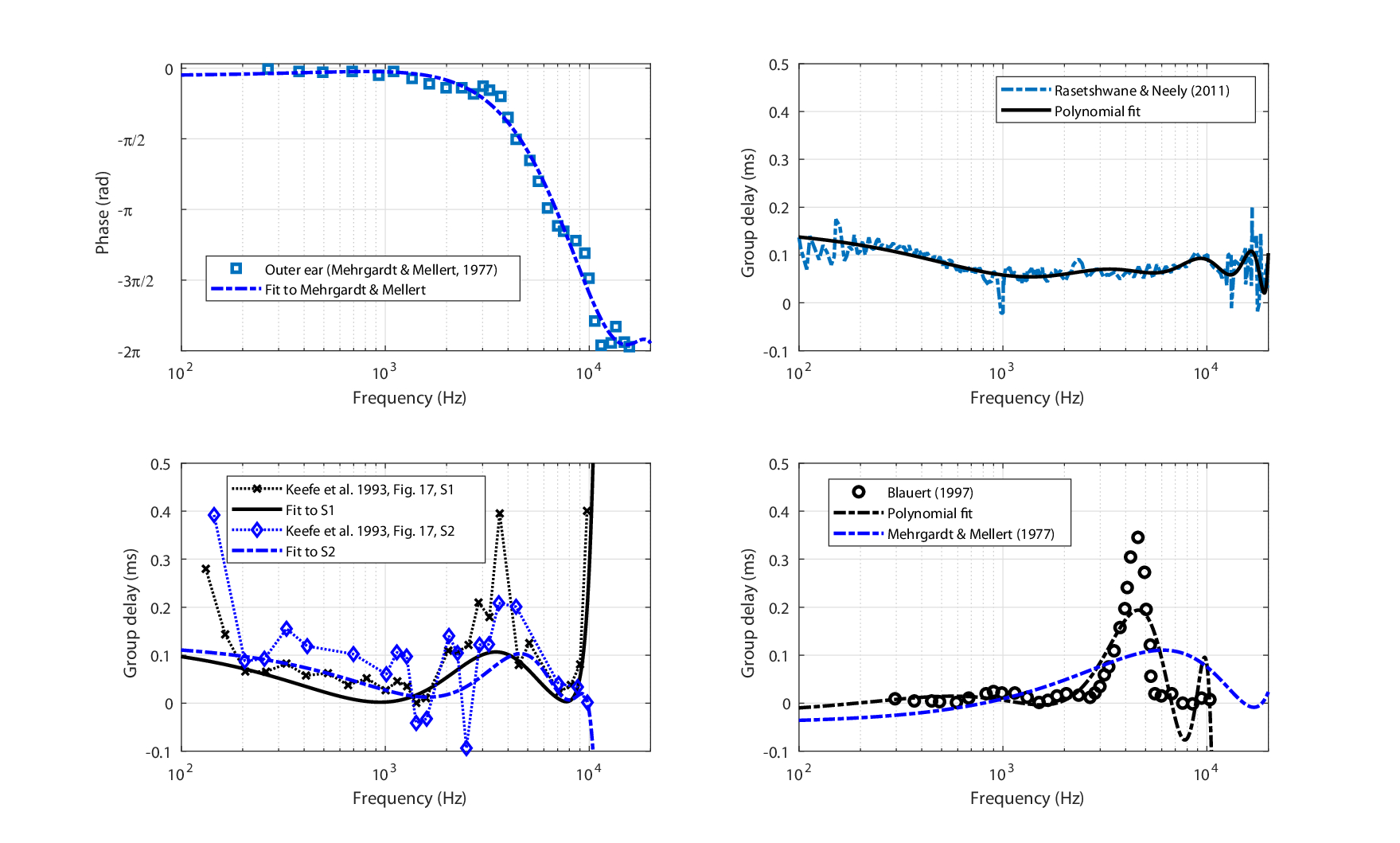
Figure 11.2: Extracted and fitted phase and group delay of ear canal data from literature. Top left: Phase response of a single subject from Mehrgardt and Mellert (1977, Figure 6, bottom), using a probe microphone at the eardrum referenced to the ear canal entrance. Top right: Group delay data based on reflectance measurements on 24 subjects (Rasetshwane and Neely, 2011; Figure 4, bottom). Bottom left: Ear canal reflectance group delay data of two subjects (Keefe et al., 1993; Figure 17, right). Bottom right: Direct ear canal group delay measurements of 11 subjects, source at 4 mm inside the ear canal, and probe microphone by the eardrum (Blauert, 1997; Figure 18, bottom, \(0^\circ\)). The bottom polynomial fits are 6th order, the top left is 4th order, and top right is 8th order.

Using the fitted phase and group delay functions, the outer ear dispersion coefficient \(u_o\) can be readily computed with

\[ u_o = \frac{1}{2}\frac{d\tau_g}{d\omega} = -\frac{1}{2}\frac{d^2\phi}{d\omega^2} = \frac{\beta^{”}_o\zeta_o}{2} \]

(11.1)

according to Eq. §10.25. The resultant group-delay dispersion from all datasets is plotted in Figure 11.3. The data exhibit large variability that reflects the relative microphone and source positions and, perhaps, the measurement methods themselves. The estimates fluctuate between negative and positive values at different spectral regions, but is bounded for \(|u| \le 1.5 \cdot 10^{-8}\) \(\mathop{\mathrm{s}}^2/\mathop{\mathrm{rad}}\). Below 100 Hz and above 10 kHz the estimates are not displayed because of insufficient data and, hence, poor fits.

The estimated values of the ear canal dispersion indicate that unless a larger and stabler group-velocity dispersion segment follows the outer ear, auditory imaging may suffer as a result of the frequent sign changes as a function of frequency.

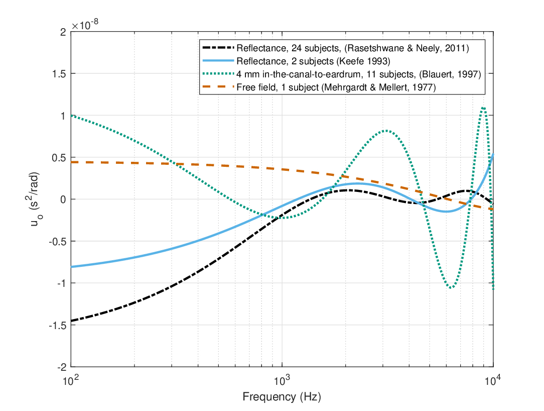
Figure 11.3: The group-velocity dispersion of the group delay data plotted in Figure 11.2, according to Eq. 11.1.

11.3 The middle ear

The middle ear appears to have relatively simple vibrational dynamics in comparison with both outer and inner ears, as its movement is essentially uniaxial and linear. While plane-wave movement is irrelevant here, the paratonal conditions can equivalently apply as long as the vibration is unimodal and one-dimensional.

11.3.1 The middle ear vibrational modes

The ossicular chain of the middle ear receives vibrational energy from the eardrum movements, which reflect the summed modes at the output of the outer ear. Measurements on human cadavers show a rather linear response in amplitude and phase of the middle ear, but they also indicate that there are several resonant modes between 1.2 kHz and 2 kHz (Homma et al., 2009). Voss et al. (2000) found that the middle ear ossicular movement is dominated by translational movement of the bones up to 1 kHz, which may be combined with additional higher-order modes at higher frequencies. High order modes are dominant at high frequencies in different animals (above 3–4 kHz in humans), where they are thought to improve sound transmission in mammals despite the ossicular mass and may even be a factor in their extended hearing range, in comparison with other vertebrates (Puria and Steele, 2010; Rosowski et al., 2020). Thus, we may also expect some level of dispersion distortion from the middle ear, which increases with frequency. Nevertheless, the frequency and phase responses generally show a linear, well-behaved transfer function of a low-Q bandpass filter centered at around 1 kHz (Voss et al., 2000; Aibara et al., 2001; Sun et al., 2002; Homma et al., 2009). Therefore, if the middle ear has any impact on the single-mode transmission, then it should appear only above 1–2 kHz and is not expected to be particularly strong. Thus, the middle ear dynamics appears to be effectively aligned with the plane-wave single mode assumption required for the temporal imaging theory. Any anomalous behavior in its response likely reflects the higher-order modes (and possibly the dispersion distortion) of the outer ear.

Note that this analysis neglects the middle ear reflex, which acts as an automatic gain control at medium-high sound pressure levels (§2.2.2). However, during fast transitions, the reflex may have a transient dispersive effect as well.

11.3.2 Middle ear group-velocity dispersion

The middle ear phase response was measured in six temporal bones of human cadavers by Nakajima et al. (2009), from which the group delay and group-delay dispersion could be calculated (Figure 11.4, left). The phase response is very close to being linear, which means that it has about constant group delay, and almost negligible group-delay dispersion. Nevertheless, a fourth-order polynomial better modeled the data than a linear fit. The polynomial fit was used to calculate the group delay (middle) and the group-delay dispersion (right), which has a smaller magnitude than the outer ear with \(|u_m|<3\cdot 10^{-9}\) \(s^2\) / rad. The linear-phase alternative produces \(u_m = 0\) throughout the spectrum, which is an unphysical result.

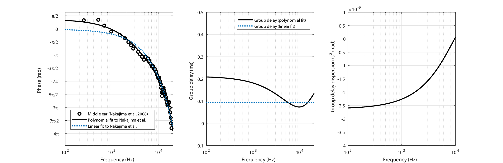
Figure 11.4: Middle ear phase response data from six temporal bones of human cadavers, extracted from Nakajima et al. (2009, Figure 5, bottom). Left: Phase response data fitted with linear and fourth-order polynomial functions. Middle: The derived group delay data, which is constant for the linear fit. Right: The group-delay dispersion is very small for the polynomial fit and is identically zero for the linear fit (not shown).

11.4 The inner ear: oval window to the outer hair cells

As the complexity of the cochlear anatomy and mechanics is much greater than both the outer and middle ears, there are several ways to segment the wave propagation before it reaches the auditory nerve. Unlike the other parts of the ear, cochlear dispersion is relatively well-documented and is sometimes considered a defining feature of the cochlear structure⁹⁹. However, the presence of the outer hair cells (OHCs) does not square with the conditions for a source-free propagation, since they generate sound through their motility (Kemp, 1978; Ashmore, 2008). Additionally, they do not constitute a passive medium for propagation, as their nonlinear amplificative nature may be taken as negative absorption, whereas the traveling wave of the passive basilar membrane itself is highly dampened within the cochlea. Therefore, the cochlear region of dispersion is defined here to include the passive path only up to the OHCs, which will be dealt with separately in §11.6.

11.4.1 Single-mode traveling wave

The cochlear fluid is forced by the oval window movement that is driven by the one-dimensional movement of the stapes footplate—the last bone of the ossicular chain. According to one of the simplest and most influential one-dimensional models of the cochlear dynamics, fast pressure waves in the incompressible cochlear fluid propagate from the oval window to the round window—first through scala vestibula via the helicotrema and into scala tympani (Peterson and Bogert, 1950). The pressure difference between the two chambers produces a much slower differential pressure wave that produces the transverse traveling wave along the cochlear partition, and specifically the basilar membrane (BM), which separates the two scalae. The fast and slow waves can be viewed as independent modes of transmission that can be expressed as plane waves. In this sense, both modes contain the acoustic information from the outside world. While the slow traveling wave theory has received most of the attention in modeling over the years (Békésy, 1960), there is still some controversy as for the exact energy balance between the two modes and the exact role of the fast wave (Robles and Ruggero, 2001). For example, there are various documented conductive loss cases where information reaches the auditory nerve, despite of a lack of a traveling waves (Sohmer, 2015), or hearing in the absence of traveling wave in the ears of lizards and frogs, which have close but somewhat different auditory anatomy and mechanisms to mammals (Bell, 2012b). The role and relative effect of the fast wave are controversial, but they appear to not be altogether negligible (e.g., Lighthill, 1981; He et al., 2008b; Bell, 2012a; Recio-Spinoso and Rhode, 2015).

Once it is transformed to a traveling wave inside the cochlea, the movement is often considered one-dimensional, although more realistic models of the cochlea are two- or three-dimensional. In the basal region before the characteristic frequency (CF) peak, most analytical models, including nonlinear ones, assume a one-dimensional wave motion with no additional modes (Zweig, 2015). This assumption is often generalized to the peak area itself, where the fluid is said to maintain laminar flow (Duifhuis, 2012; pp. 58, 109–110). In the class of solutions referred to as the “long-wave approximation” models, the geometrical distribution of the peak resonance over the width of the BM is neglected, and the velocity of the fluid around the peak is redistributed to reduce the problem to a single dimension—still giving good agreement with observations—even though the latter assumption is wrong (de Boer, 1996). While increased dimensionality in the modeling is physically essential to produce the resonance of the BM, the modeling advantage of going to three over two dimensions may be marginal (Zweig, 1991; de Boer, 1996). Higher-dimensional models sometimes treat the fluid as three-dimensional, but still assume a one-dimensional array of resonators (Zweig, 2015; Zweig, 2016), or a transmission line (Peterson and Bogert, 1950; Verhulst et al., 2012).

The traveling wave itself is usually modeled as unimodal as well, but there are indications that it may not be the case throughout the cochlea. A second mode was suspected as contributing to the nonlinear dynamics unraveled by Rhode (1971). Higher-order vibrational modes that were found useful in early modeling attempts of the cochlear partition were also considered to be a necessary ingredient of cochlear models that should account for anomalous click glides (Lin and Guinan Jr, 2004). A finite-element method (FEM) simulation of a simplified passive cochlea (a straight box model with a single partition as the BM) decomposed the traveling wave to orthogonal modes (Elliott et al., 2013; Figure 7). It was found that the fundamental mode at 1 kHz is 25–30 dB stronger than the second strongest mode. Evanescent modes became more significant only more apically than the CF (after the peak), but they decayed relatively quickly farther away. These findings are similar to Watts (2000), where some cochlear modeling inconsistencies were resolved by adding a second mode after the peak, which was also hypothesized to account for Rhode's observations.

Another assumption that is important to keep in check is the lack of dominant reflections that affect the forward-propagating waves in the cochlea. According to some evoked otoacoustic emission (OAE) models, the emitted spectrum is the result of multiple reflections from the basal end of the cochlea or from the helicotrema (Kemp, 1978). However, the existence and exact nature of such reflections are not settled matters (Kemp, 2007). For example, reflections from irregularities in the cochlear walls may interfere with the propagating wave in the BM and there is some evidence from interferometric and OAE measurements of the chinchilla that it creates ripples (micro-structure) in the BM spectrum, phase, and multiple-lobe envelope response to clicks (Shera and Cooper, 2013, but see He and Ren, 2013; Wit and Bell, 2015; Shera, 2015). While these small ripples seem to occur in many click measurements, some argue that the contribution of reflections to the overall cochlear response may be safely neglected (de Boer and Viergever, 1984). A reverse traveling wave was inferred to be present from the measurements of ex-vivo gerbil cochleas both at basal and apical positions relative to the characteristic frequency in the first and second cochlear turns (Zosuls et al., 2021).

In summary, the assumption of the single-mode transmission appears to be good only in first approximation, as it may be violated more apically than the CF peak. The exact effect of the higher-level modes or internal reflections on the neural coding and eventual perception, however, is not at all clear, especially since much of their analysis has been done in simulations, simplified theoretical models, or animals. Nevertheless, we shall assume that these effects are small enough to be negligible, while focusing on the qualitative first-order response of the cochlea in their absence. This approach is going to be surprisingly effective, despite the mitigating approximations.

11.4.2 Cochlear dispersion and group-velocity dispersion

It was Békésy (1943/1949) who first observed that different pure-tone frequencies appear with different delay between the stapes and their corresponding CF resonance on the basilar membrane. In the most immediate interpretation, the differential delay reflects the different paths that the traveling wave information takes to arrive to the peak region. The basal end of the BM, close to the oval window input, responds to high frequencies faster (it peaks earlier) than the apical end responds to low frequencies, due to the frequency-dependent impedance of the BM. A more physically rigorous explanation was provided by Ramamoorthy et al. (2010), who showed that even a simplified system with a uniform plate (modeling the BM) coupled to a fluid-filled duct exhibits dispersion. The mechanical dispersion translates to dispersion in the neural encoding of different frequencies.

As it turns out, the group delay itself is also frequency dependent as was first observed neurally in rats, where it was found that the input frequency slopes of FM tones were not conserved at the output (Møller, 1974). The change in instantaneous frequency is a characteristic of the impulse response of the basilar membrane and is referred to as a frequency glide (de Boer and Nuttall, 1997; see Table §6.1). Further direct observations were obtained in different animals, although the glide direction may vary between species and CFs (e.g., Recio et al., 1998; Carney et al., 1999; Recio-Spinoso et al., 2005; Wagner et al., 2009; Recio-Spinoso and Rhode, 2015). Pyschoacoustic confirmation for dispersion has been obtained several times as well (e.g., Smith et al., 1986; Kohlrausch and Sander, 1995; Oxenham and Dau, 2001a; Oxenham and Dau, 2001b; Summers et al., 2003; Shen and Lentz, 2009), where the curvature has been found to be negative and to increase with frequency, contrary to findings in certain animals. Oxenham and Dau (2001b) noted that the phase behavior cannot be predicted by simple auditory filter models. Indeed, inconsistent estimates of group delay as a function of frequency were computed using seven different cochlear models (Saremi et al., 2016; Figure 6A). Simulating clicks of 1 kHz carriers, the modeled group-delay slopes around 1 kHz were found to be inconsistent in sign and in their functional form (linear or curved). However, many of these studies do not make a clear distinction between dispersion arising in the cochlea itself and other dispersive contributions from the rest of the auditory system (but see §11.7.2).

While there is some inconsistency regarding the exact mechanism behind the frequency glides, as well as their exact frequency dependence in humans, there is no doubt that they exist. Although the glide slopes are not always straight, none of the cited studies advocated for phase terms that are higher than quadratic. Thus, in the vicinity of the CF, a linear curvature seems to be an acceptable assumption. This assumption will be challenged in §15.9.2.

11.4.3 Estimating the cochlear group-delay dispersion

Several attempts at estimating the group delay of the cochlea have been published that employed different methods, all of which contain rather strong assumptions that make the estimates uncertain to some extent. For example, both evoked auditory brainstem response (ABR) and evoked transient OAE (TOAE) have been used as indirect methods to estimate the cochlear group delay. For this to be the case, their output must contain exactly the same dispersive contribution from the cochlea and it should be ensured that neural group-delay dispersion is negligible. This was the conclusion of an early attempt to compare the estimates from the two methods in Neely et al. (1988), where data from separate TOAE and ABR studies were similar enough, so that the contribution of the neural pathways to the responses was considered to be a constant delay (i.e., that results in zero group-delay dispersion). However, a more recent study that repeated the comparison using simultaneous measurements of ABR and TOAE, using the same stimuli and subjects, could not establish an identical group delay of the two measures, regardless of the specific parameters used for the stimuli (Rasetshwane et al., 2013)¹⁰⁰.

A somewhat more transparent cochlear group delay estimation method was therefore favored, based on a group delay map measured in the chinchilla and transformed to human (Temchin et al., 2005; Ruggero and Temchin, 2007). In-vivo cochlear group delay was measured between the eardrum and the auditory nerve of the chinchilla using the Wiener-kernel method for obtaining the nonlinear impulse response from white noise (Temchin et al., 2005). Additional post-mortem group delay measurements of the chinchilla allowed Ruggero and Temchin (2007) to form a re-tuned map for the cochlea that could be used to transform between the live and post-mortem measurements. It was also corrected for frequency-dependent phase shifts as a result of death, which reflect the active effect of amplification in the live cochlea. Then, due to scaling similarities between all mammals and in particular the similarity between the chinchilla and human hearing ranges, the authors were able to transform human cadaver data to a live map of group delay (Ruggero and Temchin, 2007; Figure 7). The group delay was corrected also for the middle ear and constant synaptic and neural conduction delays (Ruggero and Temchin, 2007; see their Figure 8 caption). The group delay data were shown to agree with a large pool of animal data, including non-mammalian vertebrates, despite widely different morphologies.

It is arguable whether the post-mortem or the live group delay data should be used in the computation of the cochlear group-delay dispersion. The post-mortem data entails OHC inactivity that removes any amplificative phase effects from the total dispersion, which are present especially at low levels. But it also broadens the cochlear filter significantly, which has an effect that extends apically from the best frequency site and may distort the phase response. The live data, in contrast, has a normal filter response, but ostensibly includes the active OHC effect¹⁰¹. Both responses include a mechanical dispersive path associated with the IHCs, which cannot be subtracted using the available data. As it turns out, the difference between the two datasets is relatively small, although the live data seem to produce stabler results in some of the calculations throughout this work.

The group delay functions are plotted in Figure 11.5, left, for the live and post-mortem human responses. The functions are affine power-law fits, reproduced from the functions in Temchin et al. (2005, Figure 13). The live data fit (solid black) is

\[ \tau_{g,live} = 0.43 + 1.67f_{kHz}^{-0.72} \,\,\,\, \mathop{\mathrm{ms}} \]

(11.2)

where the group delay \(\tau_{g,live}\) is given in ms and the frequency \(f\) in kHz. Similarly, the post-mortem group delay function is given by

\[ \tau_{g,dead} = 0.02 + 1.85f_{kHz}^{-0.98} \,\,\,\, \mathop{\mathrm{ms}} \]

(11.3)

The cochlear group-delay dispersion \(u_c\) can be directly obtained by differentiating these expressions with respect to \(\omega\) and dividing by 2, according to Eq. 11.1 (Figure 11.5, right). Additionally, for comparison, some of the above-mentioned evoked ABR and OAE group delay data are plotted as well. The OAE is from Shera and Guinan Jr (2000) and Fobel and Dau (2004) and the ABR is from Neely et al. (1988).

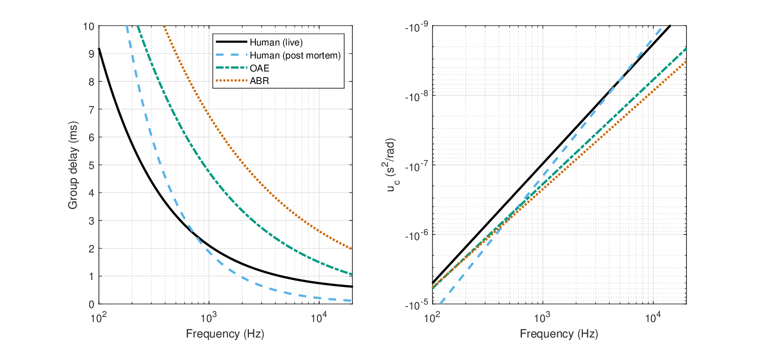
Figure 11.5: Left: Live (black solid) and post-mortem (blue dash) group delay of the human cochlea, based on human cadaver data compiled by Ruggero and Temchin (2007, Figure 7), which were corrected for the effects of death using a chinchilla group delay cochlear map from Temchin et al. (2005). Additional estimates based on closed-form functional fits are based on OAE measurements (green dash dot) (Shera and Guinan Jr, 2000; Fobel and Dau, 2004) and ABR (red dot) (Neely et al., 1988). Right: Group-delay dispersion derived from the group delay curves on the left.

11.5 Total group-delay dispersion of the inner ear

Combining the dispersions of the outer ear (\(u_o\)), middle ear (\(u_m\)), and cochlea (\(u_c\)), we can obtain an estimate for the total input dispersion of the human auditory system

\[ u = u_o + u_m + u_c \]

(11.4)

The total group-delay dispersion is plotted in Figure 11.6 both for the live and for post-mortem responses, which merge above 3 kHz. The outer ear was taken as the relatively “well-behaved” average response from Rasetshwane and Neely (2011), which was based on many more subjects than the other datasets (Figure 11.2). The middle ear data were based on the only dataset that was analyzed here from Nakajima et al. (2009).

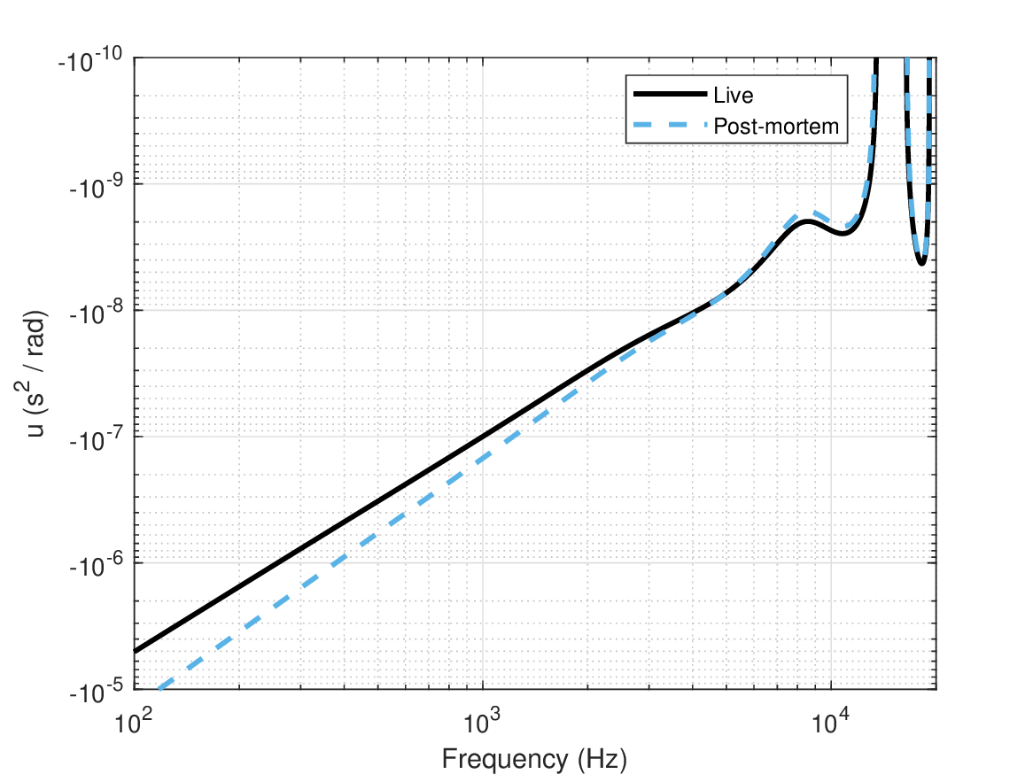
Figure 11.6: Total group-delay dispersion of the outer ear (Rasetshwane and Neely, 2011), middle ear (Nakajima et al., 2009), and cochlea (Ruggero and Temchin, 2007). The discontinuity above 10 kHz represents a sign change, where the cochlear dispersion no longer dominates the input dispersion and all three estimates are unreliable.

The most important feature of the total input group-delay dispersion is that it is mostly dominated by the cochlear group-delay dispersion. It means that it is not subjected to fluctuations in frequency caused by the outer ear acoustics. Otherwise, more sign-change “holes” in the group-delay dispersion curve could have dominated the total group-delay dispersion, as is seen at around 16 kHz in Figure 11.6. The same logic applies to the atmospheric dispersion that can be dominant in extreme weather conditions or very long distances (Figure §3.3). These effects may be absorbed by the relatively large cochlear dispersion (Figure 11.1).

Because of its dominance, we will often refer to the total input group-delay dispersion \(u\) simply as cochlear dispersion.

11.6 The inner ear: time lensing by the outer hair cells

The time lens is the second new function of the OHCs that is hypothesized in this work. The first one was of a phase-locked loop (PLL; §9). Despite their differences, the two may not be altogether independent as will be suggested in §16.4.2. However, this section, while presenting five separate lines of evidence and a hypothetical mechanism, may be rightly considered speculative—even more than the PLL—especially given that it relies on an acoustic phenomenon that has not been previously modeled (phase modulation)¹⁰². Nevertheless, the utility of this proposal will be essential for the temporal imaging theory, and hence for the rest of this work. As will turn out, the empirical evidence we have is sufficient to demonstrate that phase modulation does exist, but extrapolating its magnitude to humans will prove challenging due to several unknowns in the process. We will therefore aim to estimate the upper and lower bounds for the phase modulation in humans and later discuss how the different bounds can relate to different known responses of the ear.

11.6.1 Stiffness-dependent traveling-wave phase modulation

In the following, a general formulation of acoustic phase modulation will be proposed, which depends on stiffness variation of the medium. Specifically, a corresponding mechanism will be proposed for how phase modulation of the traveling wave can emerge as a result of the unique features of the OHCs, and by proxy, the organ of Corti. Because of the paucity of direct empirical data, it is kept largely qualitative and, arguably, oversimplified.

Let us examine the phase velocity of a narrowband disturbance, as it propagates from the base of the cochlea to its apex as a traveling wave, through the site of the CF resonance. The speed of propagation depends on the local density of the BM and its Young's modulus (or its stiffness, if it is modeled as a one-dimensional oscillator array). It is well-established that the BM stiffness (and the stiffness of other supporting cells in the organ of Corti) varies continuously and monotonically along the BM due to geometrical changes (Naidu and Mountain, 1998; Emadi et al., 2004; Teudt and Richter, 2014; Békésy, 1960; pp. 466–469). Additionally, around the resonance, the stiffness of the BM changes with the electromotile actuation of the OHCs (He and Dallos, 1999; Zheng et al., 2007), which are embedded in the organ of Corti that is attached to the BM with the supporting Deiters cells (Slepecky, 1996). When the traveling wave moves from the base toward the site of resonance, its movement gradually causes more vigorous hair bundle deflections, which in turn gate a stronger current in the OHCs and raises their intracellular potential. Apical to the resonance, the mechanoelectric activity decreases. Therefore, the somatic stiffness of the OHC is effectively modulated with the OHC potential, which in turn modulates the speed of propagation and the phase of the traveling wave in the BM. While there is some controversy about the voltage dependence of the OHC stiffness in vivo (Hallworth, 2007; Dallos et al., 2008; Liu and Neely, 2009), even a small effect can produce the phase modulation needed in a way that does not violate the observations by Hallworth (2007), who did not find significant stiffness-voltage dependence in vitro.

Let us look at a forward traveling wave around \(\omega_c\),

\[ p(z,t) = a \exp\left[i(\omega_c t - kz)\right] \]

(11.5)

Using the phase velocity definition \(c = \omega/k\), we would like to find the phase of the wave at point \(z\), which is within the region of the OHC modulation that is associated with the CF

\[ p(z,t) = a \exp\left[i\left(\omega_c t - \frac{\omega_c z_0}{c} - \varphi(z,t)\right)\right] \]

(11.6)

The instantaneous phase \(\varphi(z,t)\) is determined by the traveling wave path between \(z_0\) and \(z(t)\). The speed of sound in a fluid is defined as

\[ c = \frac{1}{\sqrt{\rho \kappa}} \]

(11.7)

where \(\rho\) is the fluid density, and \(\kappa\) is its adiabatic compressibility (Morse and Ingard, 1968; p. 229). In the case of a one-dimensional oscillator array, \(\rho\) is instead the mass per unit length, and \(\kappa\) is longitudinal compressibility—the reciprocal of stiffness per unit length \(K\) (Morse and Ingard, 1968; p. 84). It is convenient to adapt an acoustic index of refraction, which enables using a relative stiffness measure. The index of refraction \(n\) is generally defined with reference to the speed of light in vacuum (Yariv and Yeh, 2007; e.g.,][p. 10), but in the acoustic case with reference to the speed of sound in air (Kinsler et al., 1999; p. 136)

\[ v_p = \frac{c}{n} \]

(11.8)

Where \(v_p\) is the phase velocity in the medium. The speed in vacuum has no analog here, so let us instead define the index of refraction relative to the speed of the traveling wave in the passive BM

\[ n = \sqrt{\frac{\rho K_{BM}}{\rho_{BM} K}} \]

(11.9)

Realistically, it may be much easier to modulate the compressibility than the density of the medium (cf., Azhari, 2010, p. 37). In this case, the index of refraction simplifies to \(n = \sqrt{K_{BM}/K}\). We assume that the phase velocity \(v_p\) is a function of position, because of the BM-width and voltage-dependent stiffness. Putting it all together, the instantaneous phase is

\[ \varphi(z,t) = \int_{z_0}^{z(t)} k(\omega) dz = \frac{\omega_c}{c}\int_{z_0}^{z(t)} \Delta n(z,t) dz = \frac{\omega_c}{c}\int_{z_0}^{z(t)} \sqrt{\frac{K_{BM}}{K\left[z(t),V(t)\right]}}dz \]

(11.10)

where \(\Delta n\) is the change in index of refraction along the acoustical path, which is calculated in analogy to optics, and is equal to 0 at \(z_0\). The end point of \(z(t)\) may be on the BM, inside the organ of Corti, or on top of it—on the reticular lamina. In this case it is determined by the voltage- and place-dependent stiffness \(K(z,V)\). Note that to obtain the most relevant results, the coordinates must be of the traveling wave system, \(\zeta\) and \(\tau\) (Kolner, 1994a). Note also that this expression is valid in a linear medium, but within a strong negative damping medium the conditions may change and make the phase level-dependent as well (see indications for a “null-frequency” point where the cochlear phase is level-independent; Geisler and Rhode, 1982; Ruggero et al., 1997 and Palmer and Shackleton, 2009).

One implicit condition for this system to be efficient is that the voltage signal must precede the traveling wave in order to instantaneously modulate the stiffness, before it reaches the CF site. This can happen in either one of two ways. One option is for the potential to build up over time (say, within several periods) after it has been triggered by the electromotile response of the OHC from the BM—effectively sustaining a feedback loop. This option is relatively unfavorable because it requires the signal to be spectrally narrow and periodic and it prevents the system from reacting instantly. Rather, it “sacrifices” the onset of the signal, before stiffness can become modulated. Nevertheless, inasmuch as this mechanism is related to the compressive nonlinearity of the OHCs, there are indications that the compression onset is not instantaneous (Cooper and van der Heijden, 2016; see also Altoè et al., 2017). Another phenomenon that suggests it may be the case is that pitch perception from very short sinusoidal stimuli builds up over a few milliseconds, as was reviewed in §9.9.3. It was interpreted as part of the PLL pulling in time, but it may have a parallel effect also on activating the time lens.

The second option is that the electromotile response is triggered by a faster wave that deflects the hair bundle beforehand. This may happen if the bundle is sensitive to the compression wave in the fluid. Alternatively, it can happen if the traveling wave of the TM, which is connected to the tips of the stereocilia, is simultaneous but a bit faster than the traveling wave of the BM. Current data suggest that the velocities of the traveling waves in the BM and TM are comparable (Stenfelt et al., 2003; Farrahi et al., 2016), although they do not allow for conclusively determining which one leads over the other in the live cochlea.

A completely different and passive alternative cause for the production of phase modulation is if the stiffness function is frequency-dependent in a manner that is tuned according to distance from the base (i.e., according to the CF). Such a condition would effectively mean that every frequency component can be subjected to a somewhat different impedance, which changes according to the channel in which it is being analyzed. So, for example, 950 Hz component would be subjected to a somewhat different stiffness when it traverses the 900 Hz and the 1000 Hz channels. As stiffness is usually measured statically and not dynamically, there is only scant evidence for frequency-dependent stiffness in the cochlea (Scherer and Gummer, 2004; de La Rochefoucauld and Olson, 2007). This stiffness function may additionally interact with the stiffness gradient that has been observed between the different supporting cells and the hair cells within the organ of Corti (Babahosseini et al., 2022). Passive stiffness modulation may seem mathematically indistinguishable from the voltage-modulated medium that was proposed as the primary mechanism. However, this possibility seems relatively tenuous at present, if only because of the limited evidence to support it, and will not be explored further.

In conclusion, we identified a general mechanism by which the traveling wave may be phase-modulated by the electromotility of the OHCs that causes stiffness modulation. Since we do not know the actual stiffness function of the BM and the organ of Corti, this expression will provide a theoretical anchor for the underlying cause for the modulation, rather than be used analytically. Instead, we will resort to empirical data that suggest a slow modulatory effect in the cochlea that can provide the evidence for a quadratic time-lens operation.

It should be mentioned that research of stiffness modulation in non-biological systems is a topic that has received some attention, but is still relatively nascent (Trainiti et al., 2019).

11.6.2 Phase modulation evidence

Five different studies were identified in the hearing literature that can be directly interpreted as showing phase modulation in the cochleas of gerbils and guinea-pigs. Four of them are amenable to numerical phase curvature estimation (Guinan Jr and Cooper, 2008; Dong and Olson, 2013; Zosuls et al., 2021; Meenderink and Dong, 2022), whereas the fifth one will only be treated qualitatively (Cooper et al., 2018). As is discussed below, a degree of uncertainty about the precise values will accompany us for the rest of this work, which is compounded by a high likelihood that the lens curvature is variable due to auditory accommodation. Therefore, throughout this work, we may occasionally consider particular bounds of time lens values rather than a fixed value.

Negative resistance due to outer hair cell activity

What appears to be an explicit demonstration of a cochlear phase response that can qualify as a time lens was shown in the Mongolian gerbil by Dong and Olson (2013). Using a spatially-coincident voltage and pressure dual-sensor to track the BM dynamics, it was possible to estimate the temporal response of the OHCs in vivo with high precision. In particular, the phase responses of the extracellular voltage, the BM displacement, and the pressure were measured around the resonance site of 24 kHz (Dong and Olson, 2013; Figure 4). The extracellular voltage was measured in the scala typmani close to the BM (a cochlear microphonic potential), which implies that it is proportional to the intracellular voltage of the OHCs (Davis, 1965). This was indirectly confirmed in Dong and Olson (2013, Figure 3), where both evoked pressure and voltage are displayed and show a peak around the CF in the live cochlea, whereas the voltage vanished post portem while the pressure remained unchanged. It was found that below and above the CF, the displacement phase leads the pressure phase, which entails that negative resistance is in effect. Critically, the voltage phase led the displacement by about 0.4 cycles at the CF, but that lead decreased both below and above the CF (in forced oscillators, the displacement lags the force and is at quarter-cycle lag at resonance; Morse and Ingard, 1968; pp. 46–49). This is indicative that the OHCs impart power to the traveling wave, which then produces the nonlinear amplification of low-level inputs (Dong and Olson, 2013; Figure 4D). But the fact that the phase drops above CF is unlike a classical oscillator (where the voltage phase lead is expected to go to \(\pi\) at \(f \rightarrow \infty\)) and appears rather like symmetrical phase modulation that co-occurs with the forced amplification.

Figure 11.7 reproduces Figure 4B of Dong and Olson (2013). It shows the relative phase between the voltage and the displacement around a CF of 24 kHz. Similar phase data for the same frequency in another animal were obtained between the voltage and the pressure, which is itself in phase with displacement, although with varying levels of smoothness and symmetry (Dong and Olson, 2013; Figures 5E and 6). As is seen in Figure 11.7, around the CF the voltage leads by almost half a cycle, but is approximately in phase with the displacement below and above the CF region.

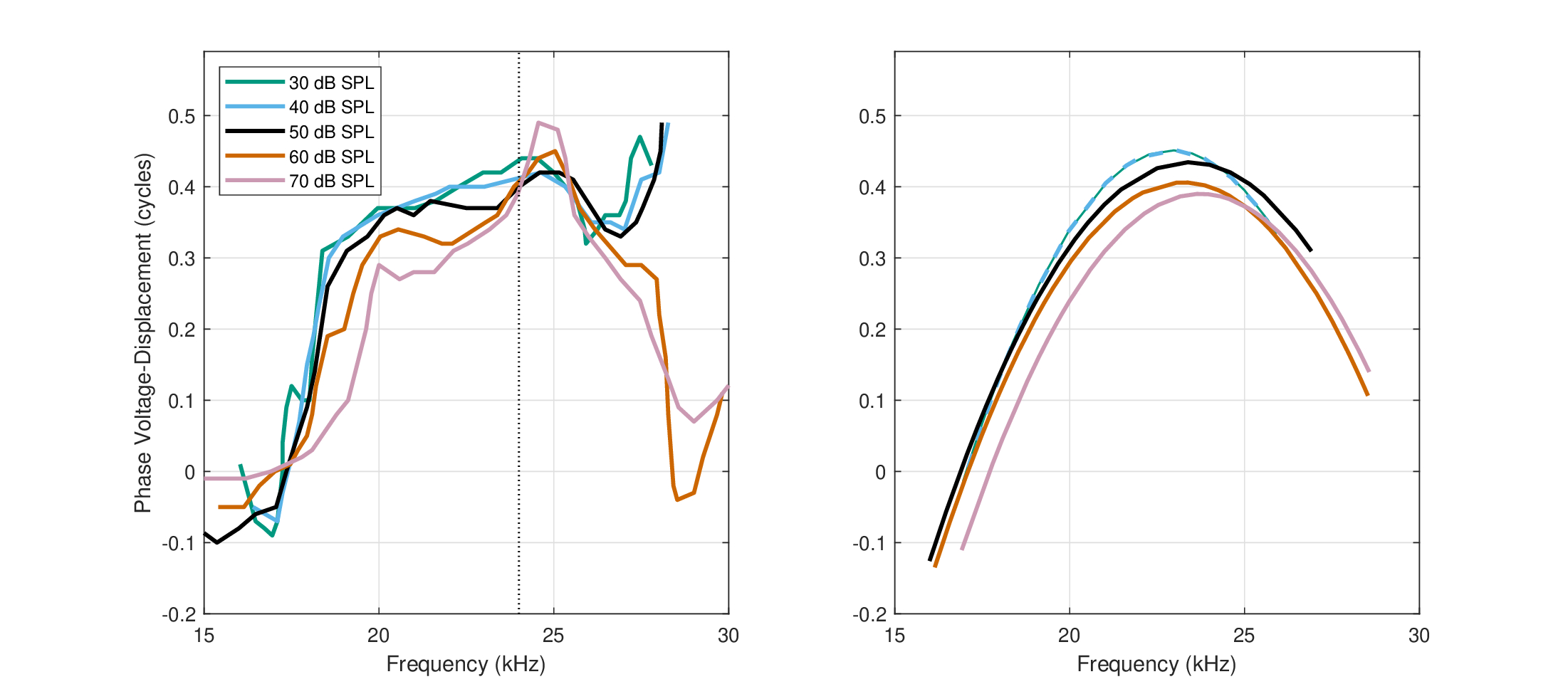
Figure 11.7: Left: Simultaneous relative voltage-to-displacement phase data of the gerbil's basilar membrane around 24 kHz at 30–70 dB SPL, as was measured by Dong and Olson (2013, Figure 4B). The extracellular voltage reflects the intracellular voltage of the outer hair cells. The displacement captures the movement of the traveling wave. Around the characteristic frequency, the voltage phase leads by about 0.4 of a cycle over the displacement. Two additional measurements at 80 and 90 dB SPL were likely contaminated by effects of the fast pressure wave modes rather than the traveling wave, which violate the measurement assumptions and are therefore not displayed. Right: Quadratic phase functions fitted to the measurements on the left. The parabola peaks were constrained to the CF in all cases.

The nonlinear phase shift appears as would be expected from a phase modulator: it has an apparent symmetrical form, which suggests that the frequency-dependent phase function may contain a quadratic component. If, as Eq. 11.10 requires, the stiffness of the OHCs is indeed voltage dependent, then there has to be a modulatory effect on the traveling wave speed at the CF, or in its propagation inside the organ of Corti. There are no direct estimates of either the stiffness or the velocity in Dong and Olson (2013), but a peak in the BM velocity can be derived from the displacement peak at the CF, as is also commonly observed elsewhere (e.g., Ren, 2002; Zheng et al., 2007). Additionally, a slowing down of the group velocity of the traveling wave at places basal to the CF was observed in vivo in the gerbil, as well as in other mammals (van der Heijden and Versteegh, 2015a). Finally, the phase variations in the BM motion just underneath the OHCs coincide with the constant phase difference observed at the reticular lamina (Chen et al., 2011; Ren et al., 2016b), although it is seen below that phase modulation may occur around “hotspots” inside the organ of Corti itself (Cooper et al., 2018)¹⁰³. Therefore, it can be deduced that any phase modulation—manifest as the difference between the extracellular voltage and displacement in the BM—should be reflected in the output of the cochlea at the IHCs and then encoded in the auditory nerve.

Indeed, auditory nerve phase measurements at low frequencies show a distinct curvature around the CF once their linear component (e.g., their mean constant group delay) is removed (or “detrended”, Temchin and Ruggero, 2010; Palmer and Shackleton, 2009)¹⁰⁴. Additionally, the curvature is often not centered around the CF (Palmer and Shackleton, 2009), and is not always symmetrical, or quadratic looking, probably depending on its cochlear position (Temchin and Ruggero, 2010). Whatever curvature was measured in Dong and Olson (2013), it incorporated also effects of adjacent dispersive paths before and after the CF. For the time being, the asymmetries that are also noticeable in the data from Dong and Olson (2013) will be ignored.

Olivocochlear efferent bundle effects

Using a displacement-sensitive interferometer to measure the vibrations of the BM, Guinan Jr and Cooper (2008) found that the phase response of a click depended on whether the medial-olivocochlear (MOC) efferent was activated (i.e., if it caused inhibition to the OHCs). A slow phase lag was observed between the onset and the first minimum of the envelope response to the click when the MOC was inhibiting compared to when it was not (no inhibition was observed in the click amplitude during the first half period). The slow change took place over several carrier cycles, so it had little effect on the instantaneous frequency of the click. We may expect that the MOC reflex (MOCR) has some effect on the time-lens curvature, perhaps in analogy to the ocular accommodation that controls the curvature of the crystalline lens. While this possibility will be explored only in §16.4.2, we shall accept it as correct, at present, and obtain estimates for the phase modulation value changes that were observed before and after efferent stimulation.

Figures 3E and 6 in Guinan Jr and Cooper (2008) display the phase difference and the zero-crossing values, respectively, of the two efferent modes for one CF in the guinea pig first (basal) turn, which allows for direct estimation of the temporal phase curvature, using Eq. §10.27. Supplementary Figures S1G and S2G of Guinan Jr and Cooper (2008) provide similar data from two other guinea pigs and CFs. The authors also stated that similar responses were obtained for the chinchilla. The apparent phase curvature, which is reproduced in Figure 11.8, covers about 60 dB of input dynamic range and seems to be level dependent. At low levels, a curvature change as a function of the MOC inhibition is hardly visible. While these measurements provide a relatively extensive dataset in the present context, it is not obvious how to extract a relevant baseline phase from it, so it relates only to changes induced by the MOC, which we assume represent the entire curvature.

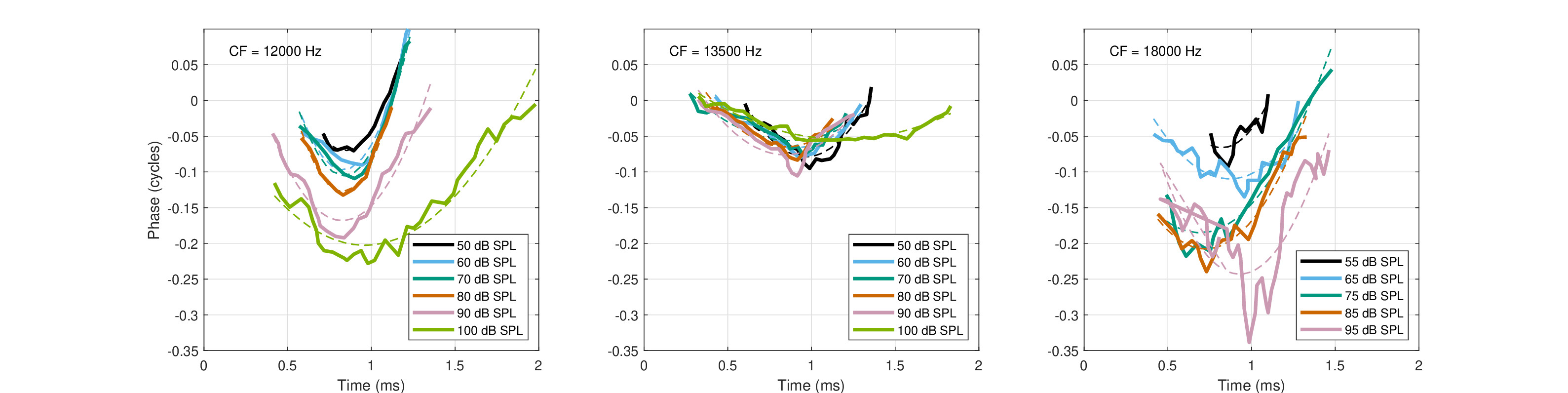
Figure 11.8: Phase response change in the guinea pig as a result of the medial olivocochlear efferent excitation at three characteristic frequencies: 12 kHz (left), 13.5 kHz (middle), and 18 kHz (right). The data are taken from Figures 3E, S1G, and S2G in Guinan Jr and Cooper (2008). The dashed lines are quadratic fits to the measurements that are shown in solid lines.

It should be also noted that Guinan Jr and Cooper (2008) ruled out that OHC stiffness change can be a likely cause of the click responses they obtained, which revealed fast inhibition (of the amplitude) after the first half cycle, whereas the stiffness changes slowly. However, the slow phase-modulation effect that we saw was predicted regardless of amplitude inhibition that may or may not appear within a few cycles. What more, the very slow phase modulation has exactly the effect we expect to have from such a nonlinear system.

Radial displacement of inner hair cell stereocilia

Traditional methods of measuring the response of the organ of Corti to external stimuli have focused on the transverse movement of the of the BM (see Figure §2.3). Using the mechanical properties of the cochlear partition, it is then possible to deduce the shear force that acts on the IHCs, which causes their movement in the radial direction. In a study by Zosuls et al. (2021), ex-vivo samples of gerbil cochlea were used to directly measure the radial motion of the IHCs, which were stimulated by mechanically actuating the BM using a probe that was placed under the outer pillar cells, and whose longitudinal position could be adjusted in increments of 2 micrometers. An inverted microscope with stroboscopic imaging and custom digital image processing were used to record the fine motion of the stereocilia in resolution of 8 nanometers. While the measurement was done on a small subsection of the organ of Corti at a time, its mechanical and biophysical properties were shown to be close enough to live animal and intact conditions, which would yield data that is sufficiently valid. We assume that the OHC section of the organ of Corti around the CFs was intact in all cases. Four measurements are presented in Zosuls et al. (2021), which provide the spatial response function of the IHC displacement, including the phase as a function of (longitudinal) distance from the CF along the BM. At four frequencies, 1 kHz, 3 kHz, 37.5 kHz, and 42.5 kHz, the phase function is presented and in all cases it shows a maximum at the CF position, in what could be well approximated using quadratic phase modulation. The relevant data is reproduced in Figure 11.9. Note that the equivalent sound pressure level that would have produced the mechanical actuation here is unknown.

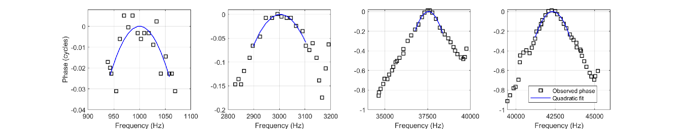
Figure 11.9: Phase data (squares) from ex-vivo gerbil cochleas, reproduced from Figures 4F (1 kHz), 4G (3 kHz), 3G (37.5 kHz), and 3H (42.5 kHz) in Zosuls et al. (2021). The original abscissas were a function of distance from the CF with a range of \(\pm 200\) \(\mu m\), but are here converted to frequency (and hence linearized), using cochlear scaling parameters from Greenwood (1990) (see Eq. §2.1 and §2.5.2). The quadratic phase fits for the points around the center frequency are plotted with solid lines. Note the different ordinate ranges of the different subplots.

Vibration “hotspots” in the organ of Corti

Using high-speed optical coherence tomography imaging of the gerbil's organ of Corti, Cooper et al. (2018) found that the vibrations between the BM and reticular lamina exhibit “hotspots” in the region between the Deiters cells and the OHCs. In phase measurements along the path between the two surfaces (the BM and reticular lamina, see Figure §2.3), the spatially and spectrally dependent phase function (relative to the BM) clearly oscillated around the hotspot, before it returned to about zero—amounting to a symmetrical phase modulation that may have a quadratic component. The degree of modulation depended on frequency and on the exact path that was imaged in the organ of Corti, which in turn determined the modes of vibration that were imaged. In one case in which a transverse path was tracked, the modulation was positive (about 0.1 cycle), tuned to the CF (23 kHz), and decreased symmetrically at lower frequencies (Cooper et al., 2018; Figure 7c). At CF of 40 kHz and a slightly different path with a longitudinal cross-section, the modulation was negative (minimum -0.15 cycles) at low frequencies, but rather shallow and mistuned at the CF (Cooper et al., 2018; Figure 8f). If these results can be generalized, then a traveling wave propagating from the BM to the reticular lamina is subjected to an internal phase modulation. Furthermore, in some cases the modulation may appear to have never happened if measured at the BM or reticular lamina alone. Similar phase patterns were also recorded in mice using related methods, only that the phase does not return to its initial value between the BM and the reticular lamina / tectorial membrane (Dewey et al., 2021; See, ][Figures 1G, 1H, and 3A).

Angle-dependence phase measurements of the organ of Corti

In a study by Meenderink and Dong (2022), the phase of the motion of the organ of Corti was measured in vivo using optical coherence tomography as a function of the angle between the laser beam and the longitudinal direction of the BM. This angle relates to different acoustic paths within the organ of Corti, whose angular dependence suggests that the OHC motion have a non-negligible longitudinal component. The phase was measured along different points between the BM and the OHCs in the second turn of the gerbil's cochlea. The angle was varied between \(-30^\circ\) and \(+30^\circ\) and produced a different frequency dependence of the phase \(\phi_{OHC}-\phi_{BM}\) in every angle, similarly to what was found in Cooper et al. (2018) and reviewed above. The phase has a clear peak, also at \(0^\circ\), which may be therefore taken to have a quadratic component, as is seen in Figure 11.10. However, as is shown in the next subsection, the curvature of the \(0^\circ\) measurement is in opposite sign to those extracted from other studies, and only at angles of \(-30^\circ\) appears to change the sign, whereas at \(-10^\circ\) the curvature becomes negligible. Furthermore, the discrepancy between the two CFs given (for both BM and OHC positions) and the phase curvature center frequency, as exists in most other measurements reviewed above, is relatively large and it is not clear which value should be used.

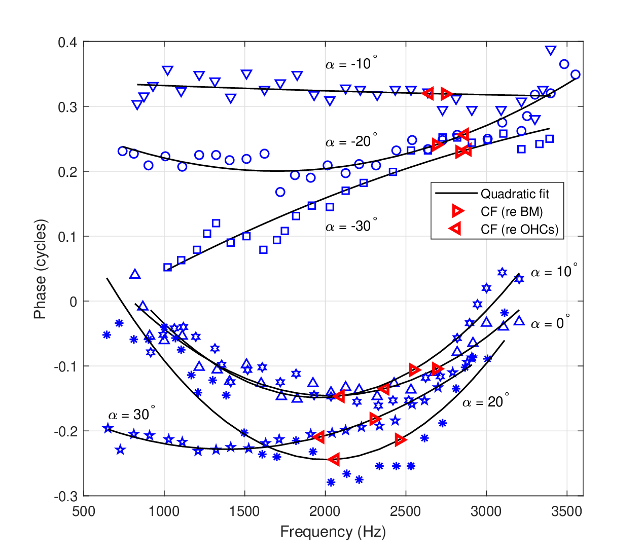
Figure 11.10: Displacement phase difference between the BM and OHC motion in the gerbil, as a function of measurement angle, and hence of longitudinal part of the trajectory in the organ of Corti. The phase data is replotted after Figure 2e in Meenderink and Dong (2022). Best frequencies for each plot was different for the BM and for the OHC site and they are marked with left pointing and right pointing red triangles, respectively, after Figures 2c and 2d in Meenderink and Dong (2022). Angles varied between \(-30^\circ\) and \(+30^\circ\), as are marked beside each quadratic plot fitted. The input level of the stimulus was 30 dB SPL.

11.6.3 Estimation of the auditory time-lens curvature

From all the studies reviewed in §11.6.2 that may be suggestive of a time-lensing function, only the phase data in Cooper et al. (2018) is directly given in the time domain. Insofar as they can be interpreted as a time lensing operation, both time- and frequency-domain representations have almost the same mathematical form (complex Gaussians, but with different signs of the argument; Eqs. §10.33 and §10.29, respectively) and thus the procedures to extract their curvatures are about the same in all cases.

Wherever reported, the phase modulatory effect is dependent on level, although the spread is small in the gerbil (Dong and Olson, 2013) and large in the guinea pig (Guinan Jr and Cooper, 2008). To constrain the spread and match it to the levels we are working with, the average curvatures were calculated from data points at 75 dB SPL or lower. Additionally, the quadratic fit was performed as a rough approximation to the curves (that were converted from cycles to radians) that change monotonically around the peak and were truncated where additional oscillations and phase shifts became visible. The resultant fits are displayed in Figures 11.7–11.10. The linear and constant terms in the fits are immaterial and were dropped in the subsequent analyses. The quadratic coefficient was readily applied in the time lens expressions to obtain the curvature and focal time in the time domain using Eqs. §10.29 and §10.32 and in the frequency domain using Eqs. §10.33 and §10.32.

All phase-curvature data and derived focal times are shown in Figure 11.11. The data can be readily clustered into two groups. High and positive curvature values \(s>3 \cdot 10^{-8}\) \(s^2/\mathop{\mathrm{rad}}\), with corresponding focal times \(f_T> 4\) ms from Guinan Jr and Cooper (2008) and Zosuls et al. (2021), and small-curvature (both positive or negative) data \(|s|<3 \cdot 10^{-9}\) \(s^2/\mathop{\mathrm{rad}}\) and corresponding focal times \(|f_T|<0.7\) ms in Dong and Olson (2013) and Meenderink and Dong (2022). While the data point at 24 kHz from Dong and Olson (2013) may be considered a mere outlier of the large-curvature group, the sign changes and very low magnitude of the rest of the data points at 2-3 kHz are completely distinct from the other low-frequency data. The low-frequency clustering may be further supported by the fact that all of these data points came from the gerbil, which otherwise yielded large-curvature values.

The large-curvature data were well fitted with a power-law model, whereas the focal time data points were nearly constant (\(f_T \approx 20\) ms) and were fitted with a linear function. However, the independent modeling of these two linearly dependent variables are inconsistent, as the curvature does not yield a constant focal point function. The other direction—of deriving the curvature from the modeled focal time—does indeed yield a satisfactory fit (if only graphically) so that this fit will be used throughout this section. The focal time for the gerbil and guinea pig is

\[ f_{T,gg}(f) = -2.06 \cdot 10^{-8} f + 0.0202 \,\,\,\,\mathop{\mathrm{Hz}} \]

(11.11)

for frequency in Hz and focal time in s. To obtain the curvature, we simply divide this expression by \(2\omega_c\) (a power law with exponent -1)

\[ s_{gg}(f) = \frac{f_T}{2\omega_c} = \frac{0.0016}{f} -1.639 \cdot 10^{-9} \,\,\,\,\, \mathop{\mathrm{s}}^2/\mathop{\mathrm{rad}} \]

(11.12)

The small-curvature data suffer from a dearth of frequency points, which may or may not be fitted with a linear function. We note that while the two animals have comparable hearing ranges (Fallah et al., 2021), it is possible that the phase measurement methods do not quantify exactly the same process or anatomy, although this seems rather unlikely. While the two clusters seem to complicate the analysis and make the data appear inconsistent, variable curvature is going to be perfectly consistent with an accommodating hearing system, in analogy to the eye. This will be reviewed in §16.

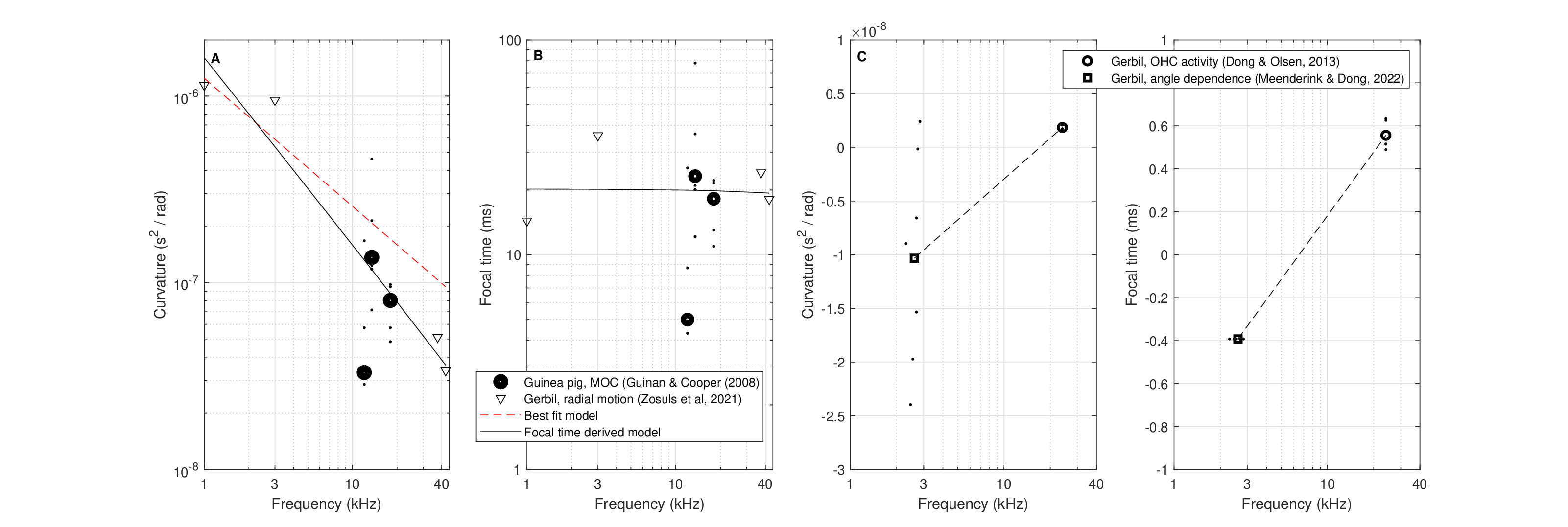
Figure 11.11: Estimated time-lens curvature (A,C) and focal time (B, D) in the cochlea of the gerbil and guinea pig, based on four independent measurements (Guinan Jr and Cooper, 2008; Dong and Olson, 2013; Zosuls et al., 2021; Meenderink and Dong, 2022). The data are clustered into two groups: large-curvature observations in panels A and B and small-curvature in C and D. Each dot marker relates to a single level/curve that appears in Figures 11.7–11.10 and whose means are marked with circle. Mean values were used to generate the power-law fit (red dotted line) for the large curvature (A) and a linear fit was used for the focal time (B). For consistency between models, an additional fit to the curvature was generated from the linear fit of the focal time and is plotted in solid black in A and is the one that is used throughout the text. Linear fits were used in C and D for the small-curvature data.

11.6.4 Extrapolation of time-lens curvature to human hearing

Short of carrying out direct measurements of the human time-lens curvature values, additional assumptions must be made in order to transform the animal data obtained to values that are valid for humans. There are several approaches that can be taken based on the available data. For example, the focal time curve appears to be approximately constant at 20 ms (large curvature). This constant may apply to all mammals, or be unique to the rather similar gerbil and guinea pig (and likely other rodents), whose data coincided. A similar option is that the focal time of 20 ms in these animals should map to the same area in the auditory brain as in humans and remain a constant. Yet another option is that the phase curvature could be scaled just like other cochlear parameters. For example, it may be scaled in accordance with the cochlear filter bandwidths that might also apply to the phase modulation function (in the previous versions of this manuscript, the latter option yielded plausible values, despite limited data). A final option is that the curvature we obtained depends primarily on the transverse cochlear geometry rather than on the longitudinal place alone (i.e., on the tissue between the BM and the reticular lamina rather than on CF alone), so it should be scaled accordingly. If a mechanism along the lines hypothesized in §11.6.1 turns out to be correct, then this last option may be the most precise. However, it depends on unknown parameter values such as the stiffness distribution in the organ of Corti, but its histological complexity (Naidu and Mountain, 1998) defies simple scaling and detailed cross-species values are not available. Therefore, this approach will not be further pursued. The three remaining approaches to derive the human curvature entail rather strong assumptions, so none of them will be completely satisfactory before they can be cross validated with other methods and data.

Constant focal time

The large-curvature data in both gerbil and guinea pig yielded a nearly flat focal time as a function of frequency, with only slight decrease at high frequencies (19.4 ms at 44 kHz), and unknown response at frequencies lower than 1 kHz (20.2 ms). This relative constancy (\(\pm 2%\)) may be a desirable feature for the auditory system, so achieving it may be a design goal that applies to all mammals. In this case we can take the same focal time curve and apply it to humans, but using the scaling property between the gerbil and human cochleas, remap it to human frequencies and find the new curvature that would produce it. The focal time in Figure 11.11 B was fitted by the linear function in Eq. 11.11. We use the very same function, but now express the frequency as a function of relative cochlear place, as is shown in Figure 11.12 D. The human focal time is then shown in Figure 11.13 B and follows the linear function

\[ f_{T,h}(f) = -5.15 \cdot 10^{-8} f + 0.0202 \]

(11.13)

The corresponding curvature is then obtained using Eq. 11.12 and is displayed in Figure 11.13 A

\[ s_{h}(f) = \frac{-5.15 \cdot 10^{-8} f + 0.0202}{4\pi f} \]

(11.14)

Analogous focal time target

A stronger assumption that may be invoked to derive the focal time is that it points to a region in the auditory system that should be analogous in the gerbil, guinea pig, and human. In evoked potential auditory electrophysiology, the 20 ms value is considered a middle latency response (MLR) potential, whose latency lies between the brainstem (ABR) and cortical potentials (Picton et al., 1974). The morphology of the MLR varies between animals, as it also depends, among others, on the individual animal, the stimulus used to obtain it, its intensity, how the recordings are filtered, and how the electrodes are placed, which itself is suggestive of multiple generators that produce some of the peaks in the MLR (e.g., McGee et al., 1991; Musiek and Nagle, 2018). The generators are thought to lie in the thalamocortical pathways, but there is also strong evidence that the inferior colliculus plays a role in the early MLR peaks (McGee et al., 1991). In the adult gerbil, three positive peaks are distinguished around the 20 ms time frame, which measured at the temporal lobe: positive peaks at 11 ms (wave A) and at 25 ms (wave C), and a negative peak at 16 ms (wave B) (Kraus et al., 1987). However, these values vary between studies, so it is not uncommon to find wave B peaking at around 20 ms and wave C at 35 ms. When measured at the midline, the morphology changes and there is a negative peak \(M-\) at -10.5 ms and a positive peak \(M+\) at 19.2 ms. The human MLR morphology is less complex and it involves a first negative wave \(Na\) with a peak at about 12-21 ms and a first positive wave \(Pa\) at about 21-38 ms, followed by second wave with \(Nb\) and \(Pb\). The exact human generators are also in doubt, but the \(Na\) is sometimes thought to arise in the midbrain (IC) (Hashimoto, 1982; McGee et al., 1991), or in the thalamocortical pathways, in which case it may be centered in the medial geniculate body (MGB) of the thalamus, as well as other subcortical regions such as the reticular formation (Musiek and Nagle, 2018).

It seems that the human \(Na\) potential is closest to the \(M-\) potential in the gerbil and guinea pig, both in generator site and in latency (McGee et al., 1991), which may suggest that \(M+\) and \(Pa\) are also analogous. Given the variance in the latencies that appear in literature for all waveforms, it will be difficult to precisely determine which latency in human would be most correctly mapped to 20 ms in gerbil, but anything between that same value and, say, 25-30 ms, may be adequate to bracket the actual focal time. This means that the above solution may be adapted as is to humans, but a range of focal times around that value may be useful to look at. As can be seen in Figure 11.13, the constant difference leads to a relatively modest change in the curvature itself.

Filter bandwidth scaling

Normally, we would like to take advantage of the scaling property of the cochlea, which enables the transformation of quantities according to their relative distance along the basilar membrane or their characteristic frequency (§2.5.2). While the CFs associated with the time lens can be transformed easily, we do not know if and how the curvature scales in the normal cochlea. However, the model that was obtained in Eq. 11.12 is a function of frequency, as are all scalable cochlear parameters. To tie the animal curvature data, different proxy variables for scaling the curvature can be conceived aside from frequency. A plausible scaling can be conjectured that is tied to the bandwidth of the auditory channel that is related to the time-lens CF, even though the time lens itself functions as an all-pass filter that needs not obey the same scaling rule as the bandpass filters. Indeed, it has been recently shown that the bandwidth does not change significantly along the active path between the BM and OHCs in both gerbils and guinea pigs—the same area that corresponds to the vibration hotspot where phase modulation seems to take place (Fallah et al., 2021; Figure 9F and 9G). As we apply this particular scaling, we are confronted by additional uncertainties regarding the correct bandwidth values that should be used for animals and human.

Guinea pig and gerbil \(Q_{10}\) spread

We can break down the uncertainty in the filter bandwidth into that related specifically to the guinea pig and gerbil and that related to humans. Conveniently, the gerbil and guinea pig have audible frequency range that appears to be close enough to one another (Figure 11.12 C; Greenwood, 1990), so combining their few available data points together was preferred here, for simplicity. Similar logic applies to the channel bandwidth, as is seen below.

Most animal frequency selectivity data are based on neural tuning curves, which directly relays the effect of cochlear processing. They are usually characterized using the 10 dB bandwidth (\(Q_{10}\)), as is plotted in Figure 11.12 A and B for the three species. For the gerbil, the most detailed auditory-nerve tuning curves data are available from Müller (1996), which reveal a substantial spread that reflect the broad sample of tuning curves and is marked on Figure 11.12 A. The confidence intervals (\(\pm\) 1 standard deviation in the plot) are nevertheless consistent with estimates based on data modeled by Kittel et al. (2002) and Ruggero and Temchin (2005), as can be seen in the figure. Unfortunately, there are almost no \(Q_{10}\) data available directly for the 37.5-42.5 kHz basal frequency range that was targeted in Zosuls et al. (2021). Therefore, while the distribution provided by Müller (1996) in tabular form was cut off at 32 kHz, the additional three data points of higher frequencies were available in his measurements and are used to form a rough estimate of the bandwidth at these frequencies. From Muller's measurements the bandwidth dependence on frequency in gerbil decreases rather than increases above 20 kHz. In similar measurements of the mouse \(Q_{10}\) a similar kink in the bandwidth curve is observed at around 30 kHz, but increases again by 50 kHz (Taberner and Liberman, 2005). Ruggero and Temchin (2005) have also provided a trend line for the guinea pig, which is quite similar to that of the gerbil—a similarity that repeats in many species regardless of their cochlear dimensions (Ruggero and Temchin, 2005). These trend lines are still contained within the confidence intervals by (Müller, 1996). Therefore, the guinea pig model will be implemented as a first-order approximation for a usable bandwidth scaling as a function of frequency (Figure 11.12 A).

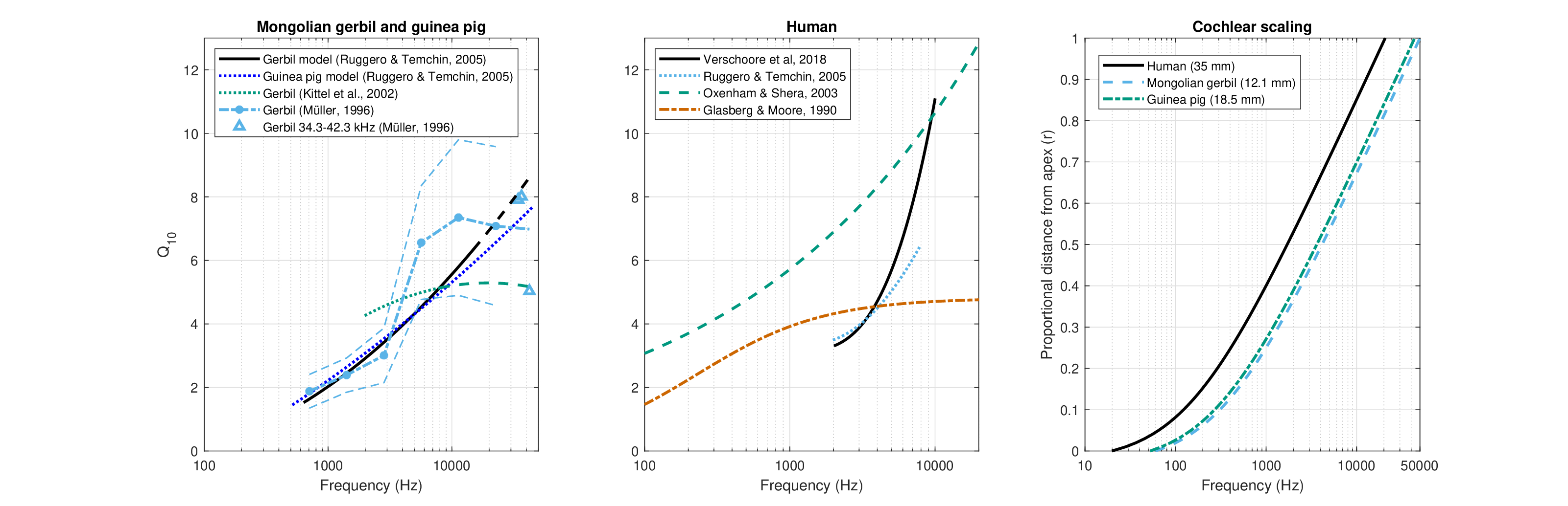
Figure 11.12: The auditory filter bandwidths, expressed as \(Q_{10}\), of the Mongolian gerbil and guinea pig, and human, as well as their cochlear scaling functions. Left: Animal \(Q_{10}\) data were collected from several sources, namely from gerbil and guinea pig models by Ruggero and Temchin (2005, Figure 6A) that are based on several auditory nerve tuning function datasets and allow for easy extrapolation across the audible range, on modeled gerbil data by Kittel et al. (2002, Figure 4), and on extensive gerbil dataset in Müller (1996, Figure 4 and Table 1), including confidence intervals that are marked with dashed lines at the \(\pm 1\) standard deviation. Middle: In humans, the sharpest filters are based on Oxenham and Shera (2003), who fitted psychoacoustic data with the power law \(Q_{ERB} = 11f^{0.27}\) (\(f\) in kHz), which can be multiplied by a factor of 0.52, to convert to \(Q_{10}\) (Verschooten et al., 2018; this factor can be also directly computed from the filter models in Oxenham and Shera, 2003). The broadest filter estimates are derived from psychoacoustic estimates by Glasberg and Moore (1990) of the equivalent rectangular bandwidth (ERB). Medium-sharp estimates are based on Verschooten et al. (2018, Figure 1) and on Ruggero and Temchin (2005, Figure 6). Right: The frequency to relative cochlear functions of the three animals based on the scaling law (Eq. §2.1) by Greenwood (1990).

Frequency selectivity in humans

While the auditory nerve tuning curves are frequently considered to be the gold standard for the peripheral filtering estimation, accessing them in humans is possible only post-mortem—after the cochlear nonlinearity disappears. Thus, the live neural tuning curves are unknown in humans and therefore require an animal reference, whose bandwidth can be compared and extrapolated between methods and species. However, the human bandwidth that should be paired with the gerbil's and guinea pig's \(Q_{10}\) is uncertain, as there has been an ongoing controversy in literature with regards to the relative sharpness of the human auditory filters. This is a twofold controversy, in fact, which relates to the absolute filter bandwidth in humans, as well as to the relative bandwidth compared to other mammals.

According to several studies, human hearing has a superior frequency resolution compared to other mammals, perhaps except for other primates (e.g., Shera et al., 2002; Oxenham and Shera, 2003; Shera et al., 2010; Joris et al., 2011; Verschooten et al., 2018; Sumner et al., 2018; Burton et al., 2018; Walker et al., 2019). Other studies found that the filters are equally sharp for all mammals (Shofner et al., 2005; Ruggero and Temchin, 2005; Siegel et al., 2005; Ruggero and Temchin, 2007; Eustaquio-Martín and Lopez-Poveda, 2011; Lopez-Poveda and Eustaquio-Martin, 2013a; Manley and van Dijk, 2016) and that they share other common features with vertebrates in general (Manley et al., 2015). These conclusions depend on the specific methods employed in each study, as well as on the theories or models used to interpret them, which in themselves are often not in consensus. For example, some results rely on stimulated-frequency OAE data (Shera et al., 2002) or spontaneous OAE (Manley and van Dijk, 2016), which require a theory to interpret them. Another example is from studies that involve either simultaneous masking or forward masking in notched-noise data, which requires control of nonlinear suppression and level dependence, as well as a clear understanding of the operation of central processing (Oxenham and Shera, 2003; Ruggero and Temchin, 2007; Eustaquio-Martín and Lopez-Poveda, 2011; Lopez-Poveda and Eustaquio-Martin, 2013a; Verschooten et al., 2018). Yet other experiments relied on pitch discrimination tasks that require some involvement of central processing as well (Shofner et al., 2005; Walker et al., 2019).

Some human \(Q_{10}\) modeled data from different sources are presented in Figure 11.12 (middle), which highlights the two extremes of sharp and broad filtering. Both the bandwidth and the frequency dependence are markedly different between studies. Sharp filter responses were found in Oxenham and Shera (2003) using forward-masking notched-noise psychoacoustic experiments, which contrast with broad filters based on simultaneous-masking notched noise by Glasberg and Moore (1990). Additional compound action potential data from Verschooten et al. (2018, Figure 1) are plotted, exhibiting sharp filters at high frequencies and broad filters at low frequencies. Modeled tuning curve \(Q_{10}\) by Ruggero and Temchin (2005, Figure 6) are displayed as well, showing broad filters, along with extrapolation to 20 kHz¹⁰⁵.

Human time-lens curvature estimation

The short reviews above indicate that there are several possible combinations of animal-to-human scalings that can be invoked to derive the human time-lens curvature, but none that is clearly more correct than the others. We will therefore aim to bracket the time-lens curvature in human and then explore the curvature-space, as needed, throughout this work. To simplify this procedure, we will use a single curve for guinea pig and gerbil filter sharpness and apply the broad human tuning according to Glasberg and Moore (1990) and the sharp tuning from Oxenham and Shera (2003). The following first applies the scaling only the large-curvature estimates (Figure 11.11 A and B). The small-curvature estimates (Figure 11.11 C and D) for humans rely on less data and are simply down-scaled in frequency from the animal data, as is presented below.

Large-curvature scaling

In order to perform scaling of curvature, we will apply the following procedure in all cases. The quality factor definition of a bandpass filter is \(Q_{10} = f_c/\Delta f\), where \(f_c\) is the center frequency and \(\Delta f\) is the bandwidth of the filter at 10 dB down from its peak. If the animal's bandwidth is \(\Delta f\), for a given \(Q\), then we can compute the bandwidth-phase pair \((\Delta f, \phi_{\Delta f/2})\) from the quadratic phase function fits around \(f_c\) (Figure 11.11). The argument of the time-lens transfer function (Eq. §10.33) in the (one-sided) bandwidth corner frequency around \(\omega_c\) is: \(\omega^2 s = 4\pi^2 (\Delta f /2)^2 s = (\pi\Delta f)^2s = \phi_{\Delta f/2}\), where \(s\) is the animal's lens curvature. Therefore,

\[ \phi_{\Delta f/2} = (\pi\Delta f)^2 s = s \left(\frac{\pi f_c}{Q}\right)^2 \]

(11.15)

Next, we would like to use the obtained animal's phase values \(\phi_{\Delta f/2}\) for the human's equivalent CF and \(Q_{10}\) and extrapolate it from there for the entire spectrum using scaling. This can be done by using one of the modeled animal bandwidths from Figure 11.12. We shall use the Müller (1996) \(Q_{10}\) data at frequencies above 1200 Hz, which extend all the way to 42.5 kHz (albeit with very few data points), but use the Ruggero and Temchin (2005) function at lower frequencies in order to obtain smooth extrapolation.

The calculation is repeated twice for the two different human filter types. First, the broad human filter bandwidth are, using the ERB approximation by Glasberg and Moore (1990)

\[ \Delta f_{h,broad} = \frac{\mathop{\mathrm{ERB}}}{0.52} = \frac{0.108f + 24.7}{0.52} = 0.208 f + 47.5 \]

(11.16)

with the subscript \(_h\) designating human values, and the conversion factor 0.52 was introduced to obtain the equivalent 10 dB bandwidth (Verschooten et al., 2018) and can be gathered directly from the filter models in Oxenham and Shera (2003). Second, for the sharp filter relations, using the approximation from Oxenham and Shera (2003) and the same correction factor

\[ \Delta f_{h,sharp} = \frac{f}{Q_{10}} = \frac{f}{0.52 Q_{ERB}}= 1.129 f^{-0.73} \]

(11.17)

Finally, using these relations, we can plug in the argument of the time lens again in

\[ s_h = \frac{\phi_{\Delta f/2}}{(\pi\Delta f_h)^2} \]

(11.18)

This curvature applies now to a new CF that has the same proportionate distance on the human's cochlea as the one on the gerbil's, according to their respective Greenwood function (Eq. §2.1) (Greenwood, 1990). It allows us to compute the human's focal time using \(f_T = 2\omega_c s_h\). In all cases we have to carry over the sign of the curvature from the animals to humans—a positive curvature both in the gerbil and in the guinea pig cases (the arguments in the frequency and time domain time lens representations have opposite signs).

The large-curvature results are displayed in Figure 11.13. They show a large spread of possible values of curvatures and focal times that are easily one order of magnitude apart between the constant-focal-time model and the various scaled models. However, the spread tends to be largest the lowest and highest frequency ranges, where the estimates rely on extrapolation and are much less reliable. Interestingly, the constant focal-time curvature estimate of 20 ms nearly coincides with the broad-filter curvature that was computed based on scaling at frequencies above 2000 Hz. The choice we made about the animal filter data made the bandwidth function jagged and the scaled curves non-monotonic.

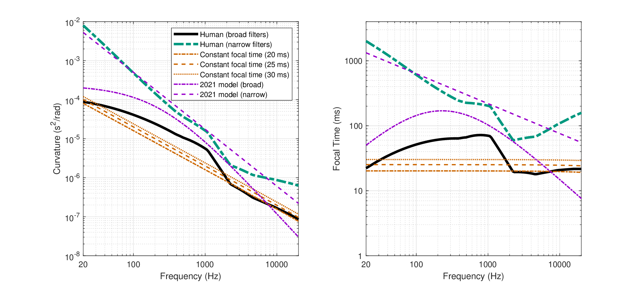
Figure 11.13: Human large-curvature mode time-lens estimates (left) and their respective focal time (right) based on different combinations of animal and human filter bandwidths and different modeling assumptions. The first two curves are calculated based on gerbil to human data scaling of the \(Q_{10}\), derived from data by Müller (1996) at high frequencies (\(>1200\) Hz), and an extrapolated model by Ruggero and Temchin (2005) at low frequencies (\(<1200\) Hz). The solid black curve applied the human broad auditory filters based on Glasberg and Moore (1990) and the narrow filters in dash-blue on Oxenham and Shera (2003). The next three curves in red are based on the assumption that the nearly constant focal time of the gerbil applies to humans, as is with \(f_T = 20 ms\) (dash-dot), \(f_T = 25 ms\) (dash), and \(f_T = 30 ms\) (dot). The last two curves are based on an earlier estimate of the curvature, when fewer data points were available. They were also based on scaling according to \(Q_{10}\) and are plotted in purple dash-dot for the broad filters in humans and dash for the narrow filters.

Small-curvature scaling

The small-curvature estimates in Figure 11.14 are based on simple scaling of the frequencies between the animals and humans of the two-point data obtained above, using the respective gerbil and human scaling functions from Greenwood (1990). Here the focal time and curvature are usually very close to zero and negative (\( -0.1 < f_T < -0.5 \) ms), which is 2-3 orders of magnitude lower than the large-curvature mode estimates.

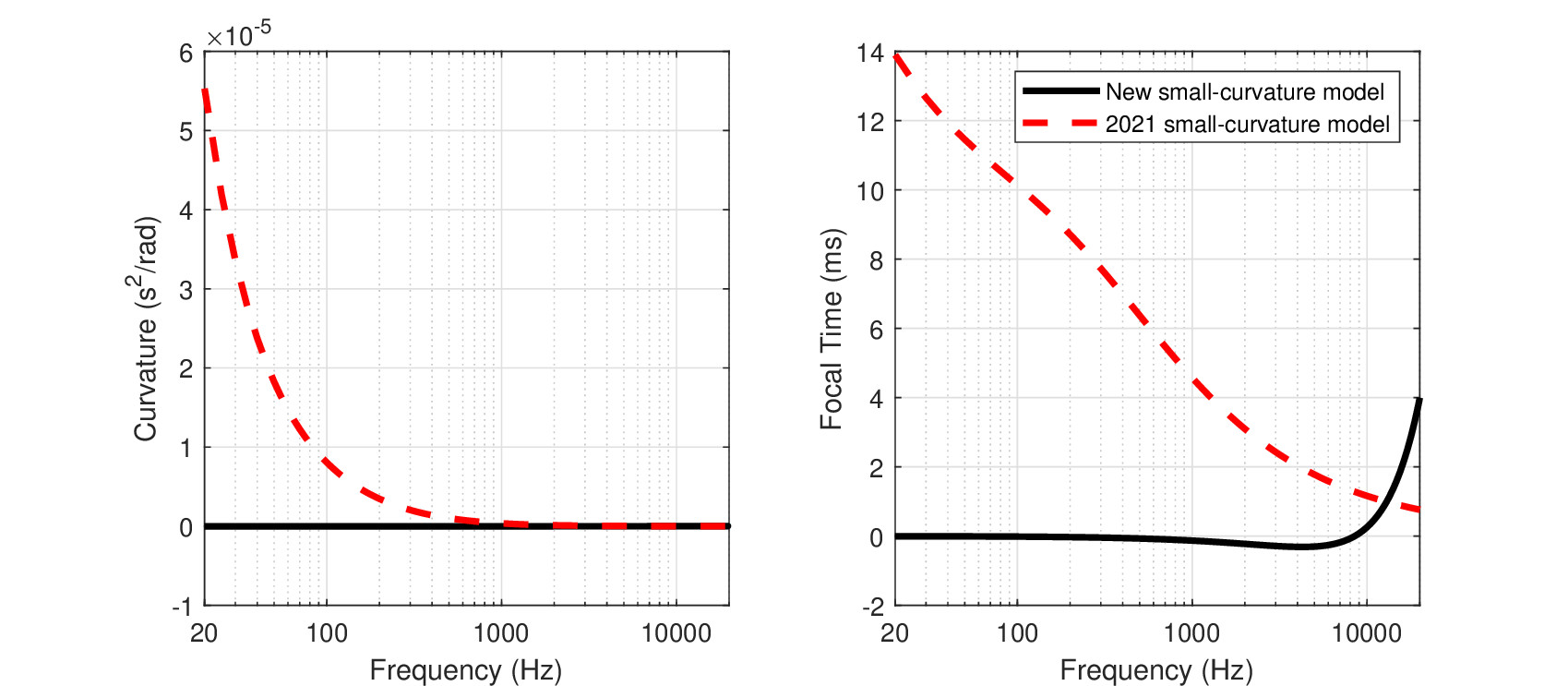
Figure 11.14: Human small-curvature mode time-lens estimate (left) and its respective focal time (right). As bandwidth scaling does not seem to apply to this limited dataset, the animal data was simply scaled (translated) to human frequencies with curvature (left) and focal time (right). The old small-curvature model from the previous version of this that applied to the one data point from the gerbil at 24 kHz is shown in dashed red for comparison and shows stark difference in magnitude and sign.

We will subsequently refer to these two estimates as the small-curvature time lens the large-curvature time lens.

11.6.5 Discussion

While we were able to obtain estimates for the time-lens curvature that will turn out to be plausible later in this work, this section may have been one of the most speculative part in the entire work (not a small feat, admittedly). This is despite the relatively simple physical model it alluded to, given the variable stiffness of the BM.

According to the above analysis, the time lens is effectively a result of an active and nonlinear function in the organ of Corti, which is naturally associated with the electromotility of the OHCs. This explanation may coincide with recent physiological and psychoacoustic findings by Nuttall et al. (2018), which conclusively determined that the place of envelope information generation is found within the organ of Corti—between the BM and the reticular lamina—as a consequence of its nonlinear distorting properties. This is exactly the effect we would expect to see following a time lens—effectively a nonlinear phase modulator.

Inasmuch as phase modulation depends on the OHCs, their number in the healthy organ of Corti of the different animals is substantially different: 11000–16000 in humans, 4600 in gerbils, and 2400 in guinea pigs (§2.5.2). While we do not know the exact effect of these large differences, they may impact the stiffness and its variability, and hence the degree of phase modulation that the OHCs can generate.

Identifying a basic time lens mechanism and obtaining estimates of its magnitude will turn out useful throughout this work, despite the inevitable lack of certainty in the estimation. It should be recognized that a very simple imaging system may be designed without a lens altogether—a pinhole camera that has only a small aperture instead of a lens (§4.2.1)—so the possibility that the auditory system might be lens-less after all will be considered at several points later on.

Another challenge to the time lens is that its effect is not apparent in the auditory nerve and other measurements. It may be because it is too small, too short, too slow, or too localized. The choice of stimulus may also be critical in observing the time lens effect anywhere beyond the organ of Corti. The effect of the phase modulation is subtle in the time domain when measured in the auditory nerve because of the limited duration of the temporal aperture—a feature of the system that is coupled to the filter bandwidth and will be examined in later chapters in detail.

At least three things were neglected in the derivation of the lens that should be eventually corrected in more refined analysis: compressive nonlinear dependence on level, asymmetry of the curvature with respect to the carrier (or CF), and phase function components that are higher-order than quadratic—perhaps contributing to the asymmetry. These will be briefly explored in §15.9.

The values obtained for the focal time of the lens can be interpreted as the additional group delay that would be required to cancel out the effect of the lens after the wave left it (Kolner, 1994b). Given that the input curvature is relatively small and the distances between the auditory nuclei are short, the highest values obtained in the focal-time range of some models (\(>\) 100 ms) appear to be grossly overblown to be compensated for by dispersion, as would be expected from an imaging system in sharp focus (§12). However, the interpretation of the extreme values is going to turn out to be nontrivial, as it does not follow the same design logic as the eye.

It will be argued much later in this work that the lens curvature is variable by design through accommodation in both visual and auditory systems. Accepting that the time-lens curvature (and associated effects) may be variable poses a complicating factor to modeling, though, because we do not know what is the “relaxed” or “normal” position for the time lens. In the spatial lens of the eye, this position is referred to as emmetropic whereby the lens focus is set to “infinity”. Effectively, objects that are 6 m or farther from the eyes are at infinity (e.g., Charman, 2010).

While we do not know what was the root cause for the difference between the animals that exhibited small-curvature vs. large-curvature time lens estimates, it is not impossible that the state of the accommodation at the time of measurement had that effect, although with unknown experimental conditions that have led to it. Hypothetically, this is supported by the study by Guinan Jr and Cooper (2008), whose results were used to derive large-curvature values in §11.6.2. The only obtainable data from that study was relative, but we used it as absolute curvature for lack of an absolute reference. The corresponding underlying assumption in doing so is that the uninhibited MOC produces nearly zero curvature. This is not too different from the small-curvature values we got, which fluctuated around zero.

Finally, the physiological mechanism of achieving phase modulation that was explored here is yet another function that is stacked on the organ of Corti, in addition to the PLL that was examined earlier. The two functions do not necessarily have to interact and they may be realized by different parts of the organ of Corti or the OHCs. Specifically, the phase modulation may be a result of the bottom part of the basilar membrane, whereas the PLL is dependent on the hair bundle and a specific feedback path through the OHC soma. Both functions assume a role for the somatic motility of the OHCs, which supplies power either to the PLL loop gain, and to the stiffness modulation. Independently, the operation of the OHC is thought to utilize the very same mechanisms to achieve its amplification function.

11.7 Neural dispersion

Having estimated the dispersive properties of the BM and the OHCs, we are left with the final part of the periphery—the IHCs and the auditory nerve—before entering the central nervous system at the brainstem. In a single-lens imaging system, as the auditory system likely is, this segment behind the lens is most conveniently modeled as a single dispersive unit. This is true even if it combines several media with different dispersive properties (as is the cochlear group-delay dispersion \(u\)), for the reason that dispersion is mathematically additive (see §B.3). However, the transduction of the sound wave to neural action potentials represents a fundamental departure from the more explicitly-physical mechanical waveforms.

Different paradigmatic approaches are common in the modeling of the acoustic-to-neural transduction. In signal-processing-oriented models, the hair bundle motion and neural transduction coupling are usually accounted for by signal rectification and low-pass filtering, while still treating the signal as continuous. These two operations entail amplitude demodulation, or (real) envelope extraction (§5.3.2). As the paratonal equation is already framed in the modulation domain, these operations may be neglected, as long as the carrier informs the envelope. In other words, tonotopy dictates that even a demodulated response would always be associated with its high-frequency carrier. The approach in neuroscience is usually to conceptualize neural transduction as a coding operation, which emphasizes the representational transformation that the physical referent (e.g., the mechanical wave) undergoes (Perkel and Bullock, 1968). Instead, in the present work, we would like to employ a more primitive operation that conceptually precedes coding (in the informational theoretic sense)—sampling. This ensures that information is conserved in the process through discretization, which can also provide several insights into the system processing for later (see §14 for a more in-depth discussion). It simplifies the discussion by avoiding coding intricacies such as the spontaneous rate of the different auditory fiber types (high, medium, or low; Liberman, 1978).

11.7.1 The inferior colliculus is the candidate auditory retina

Having delineated its reach and contents, the analysis of the final segment of the dispersive path of the sound signal boils down to a single question: what is the destination of the signal? Or alternatively—if a complete imaging system view is adopted (as will be shown in §12)—what is the “screen” on which the final image is “projected”? Candidate areas can be argued for given their key roles in auditory perception and processing: the auditory nerve, the cochlear nucleus (CN), the inferior colliculus (IC), and the primary auditory cortex (A1). We would like to argue that the IC is the destination and its role can be likened to an “auditory retina”¹⁰⁶. There are several arguments that can be made to support this claim, each from a different standpoint. The first two arguments complement those that were made in §1.5.2:

1. Anatomical analogy—The retina is where an optical image is formed, which the visual system can then process, whereupon it culminates in visual perception. The retinal connection to the brain is unique among the peripheral senses, because the second cranial nerve (the optic nerve), which connects to the retinal ganglion cells, is in fact part of the central nervous system that projects from the forebrain (Rea, 2014; pp. 7-10). Specifically, the optic nerve is projected from the lateral geniculate body (LGB) in the thalamus and from there to the visual cortex in the occipital lobe. Only a small fraction of the optic fibers bypass the LGB and lead to the pretectal nucleus and to the superior colliculus (SC)—two midbrain structures that are responsible for various reflexive visual functions. In analogy, the primary projection from from the IC is also to the thalamus—to the medial geniculate body (MGB), which is considered the main nucleus between the IC to A1 (Malmierca and Hackett, 2010). Incidentally, some of the IC subnuclei project to the SC and the pretectal nucleus as well (Kudo and Niimi, 1980). More intricate analogies between the IC and the retina exist, based on function and processing (Kvale and Schreiner, 2004).
2. System physiology—All information from the CN, the superior olivary complex (SOC), and the lateral leminiscus (LL) converges in the IC (Aitkin and Phillips, 1984; demonstrated on the cat), with very few exceptions of fibers that directly project from the CN to the contralateral MGB (see Figure §2.4). Its importance is also manifested in the number of neuron cells it has compared to other subcortical auditory structures—an average of 373,000 in the rat, which is one or two orders of magnitude more than in the CN, the SOC, the LL and the MGB (Kulesza Jr et al., 2002). Also, the IC appears in the auditory system of all mammals and in birds (Casseday and Covey, 1996), and has a homologous structure (the torus semicircularis) in the midbrain of amphibians, reptiles, and fish (Bass et al., 2005). Finally, out of all the brain structures (including all auditory nuclei), the glucose metabolized by the IC is the highest—about twice as high as the superior colliculus in rhesus monkey (Kennedy et al., 1978) and in albino rats (Sokoloff et al., 1977).
3. Function—Another unique feature of the IC is that different signal processing pathways converge to organized maps that share the same tonotopy. In the IC, tonotopic maps are organized in characteristic iso-frequency laminae, which are thought to be orthogonal to a further map of periodicity that is then propagated to A1 (Langner, 1997). This property of the IC suggests that the information necessary for cortical processing is complete at that stage, even if certain dimensions (e.g., spectral, temporal, and spatial) of the stimulus are separately processed downstream.
4. Information—The coding of the modulation transfer function in the brain distinctly shifts in the IC to a rate code from a temporal code that is more characteristic in the CN and SOC (Casseday and Covey, 1996; Joris et al., 2004). It suggests that a maturer degree of signal processing may be possible at this stage, which was unavailable in the brainstem nuclei. It may be deduced, for example, from studies in bats who could still echolocate in part after the ablation of their A1 (Suga, 1969a), but not at all after ablation of their ventral IC (Suga, 1969b). From a system design point of view, it seems efficient that there should not be a change in coding before the imaging process is complete.

11.7.2 The existence of the neural dispersion

We would like to estimate the dispersion of the auditory signal path from the back of the time lens—presumably in the organ of Corti at the reticular lamina before being coded in the IHCs—all the way to the IC. This should include the effects of the auditory nerve and the IC, as well as the intermediate pathways in the brainstem. Unfortunately, it will be impossible to isolate the response of the IHCs from the previously calculated live cochlear dispersion. The synaptic delay of the auditory nerve is often taken to be constant (e.g., Palmer and Russell, 1986; Ruggero and Rich, 1987), which would mean that its group delay and group-delay dispersion are both zero. This leaves us with the dispersive contribution of the auditory nerve fibers and the central nervous system as the dominant component of this dispersion. Hence, we refer to it as neural dispersion, even though it begins in the cochlea.

Neural dispersion has been hypothesized a number of times in the past (e.g., Neely et al., 1988; Fobel and Dau, 2004; Harte et al., 2009), but was ruled out more often than not. For example, Neely et al. (1988) estimated the difference between the latency of wave V in ABR and OAE measurements of two evoked-response datasets with similar tone-burst stimuli (Gorga et al., 1988; Norton and Neely, 1987). In theory, the ABR includes both the mechanical and neural pathways, whereas the OAE response includes only (approximately double the) mechanical path (more about it below). The group delay was estimated according to the two measurements and a good match was obtained to within \(\pm2\) ms (Neely et al., 1988; Figure 3). The two estimates were assumed to differ mainly due to the neural pathway that has a constant delay. The authors postulated that any significant neural effect is practically eliminated at low stimulus levels, as the two measurements differ only by a frequency-independent delay. Indeed, the ABR and OAE group delay measurements appear to have converged. In another example, the group delays of waves I, III, and V were compared using derived-band ABR and were found to vary by a constant, which implied that they are determined by the auditory nerve alone and any frequency-dependent group delay propagates downstream from there, unchanged (Don and Eggermont, 1978).

Even though auditory neural pathways may appear to be dispersionless, they are physical transmission paths and as such must have a finite dispersion. To the best knowledge of the author, the only data that explicitly demonstrate it is from a study by Morimoto et al. (2019). The objective of that study was to maximize the peak response of either wave I or wave V of a chirp-evoked ABR measurement, which was designed to compensate for the cochlear dispersion and concentrate as much energy as possible at the peak of wave V (Elberling and Don, 2010)¹⁰⁷. Using data from 25 normal-hearing subjects, different chirp slopes were found that maximized the two wave peaks, albeit with large individual variation. It suggests that the path between the areas that corresponds to wave I (the auditory nerve) and wave V (the contralateral LL or the IC) is (group-delay) dispersive¹⁰⁸. Note that these frequency-dependent differences between wave I and wave V delays were not reliably reproduced, as observed using the same chirps and other click stimuli in derived-ABR measurements by (de Boer et al., 2022). If neural dispersion difference between waves I and V appeared at all, it was relatively small (especially on the group level) and its effect was not monotonic in frequency.

More indirect evidence for neural dispersion can be gathered from octopus-cell recordings in the mouse by McGinley et al. (2012). The octopus cells in the posteroventral cochlear nucleus (PVCN) work as broadband coincidence detectors (§8.5), where dendrites from different cochlear locations converge. The different dendrite lengths compensate for the across-channel delay that is caused by the cochlear dispersion and thereby allow for the temporally precise detection to take place, effectively time-compressing the broadband output from the cochlea¹⁰⁹. As these findings apply only to one specific cell type and function, it is unknown at this stage if and how they should be generalized to the other brainstem nuclei. This may be reinforced by findings from the big brown bat, which showed that tuned units had a range of latencies that grew from the CN (smallest) to the LL, and through to the IC (largest) (Haplea et al., 1994). These differential delay lines inevitably create neural dispersion, although with patterns that may be difficult to pin down using a single parameter.

Simultaneous measurements of evoked ABR and TOAE may be also used to show the existence of neural dispersion, as there is generally a small but consistent difference between the slopes of the two. An example of this difference was displayed in Figure 11.5, where the unused OAE and ABR estimates of cochlear group delay and group-delay dispersion are plotted. If the two represented only cochlear dispersion, as standard theory has it (e.g., Neely et al., 1988), then they would only differ by a constant delay that does not affect group-delay dispersion. However, their slopes are different, which means that their group-delay dispersions are frequency dependent and different from one another. This subtle difference opens up the possibility of computing the neural dispersion from the difference between these ostensibly identical estimates of the ear's group delay. Hence, differentiating the group delay difference between ABR and OAE measurements (using Eq. §10.25) should give us the neural group-delay dispersion \(v\)

\[ v = \frac{\beta_2”\zeta_2}{2}= \frac{1}{2}\frac{d}{d\omega}(\tau_{gABR} - \tau_{gOAE}) \]

(11.19)

where the frequency-dependent group delay of the ABR is \(\tau_{gABR}\) and of the OAE is \(\tau_{gOAE}\).

To make things more complicated, though, the interpretation of the various types of OAEs, the TOAE amongst them, requires a model that identifies both the generator and/or the source of reflection in the cochlea that accounts for the return travel time of the emission. As in other cochlear research questions, there is no universal agreement about these issues. The main point of controversy is determining whether different types of evoked OAEs occur due to reflections from irregularities in the cochlear geometry and mechanics, or rather from active nonlinear mechanisms that act as sources, or some combination of both (e.g., Probst et al., 1991; Shera and Guinan Jr., 2008). It appears that both reflection and nonlinear models identify the OHCs as the site of (re-)emission. Even then, there remains an additional uncertainty regarding the return path of the reverse wave, which is factored into the group delay estimation. If a reverse wave returns through the BM, then we can expect that the group delay is double the forward path, \(\tau_{OAE}(\omega) \approx 2\tau_{BM}(\omega)\) (Shera and Guinan Jr, 2003). However, in species where the group delay could be measured directly from the mechanics, it turned out smaller than this prediction (e.g., for the chinchilla the factor is 1.86 instead of 2; Cooper and Shera, 2004). It suggests that at least some of the energy may be returned to the middle ear in another (faster) path different from the forward path. In the present context, the important distinction is between an OAE measurement that includes or excludes the dispersive contribution of the phase-modulating organ of Corti, both in the forward and reverse paths. While resolution of this controversy is beyond the scope of this work, using the OAE in Eq. 11.19 as though it includes the time-lens curvature seems to work reasonably well and does not require a correction at this stage. However, we note that there is an unknown error expected using the general method of the neural dispersion estimation based on Eq. 11.19.

11.7.3 Neural dispersion estimation

The neural dispersion will be estimated here based on Eq. 11.19 and on the small but persistent difference in group delay of ABR and OAE measurements found in literature. Comparable measurements of OAE and ABR were reported several times, but despite the qualitative similarity of the results, they are numerically inconsistent. This inconsistency is exacerbated upon differentiation, which is where group-delay dispersion arises.

The OAE and ABR measurements by Neely et al. (1988) were originally fitted to a level-dependent power law that has also been adopted in several other studies later (see also Anderson et al., 1971)

\[ \tau_g = a + bc^{-i}f^{-d} \]

(11.20)

where \(i\) is the ratio of the input in dB SPL to 100 dB SPL, and \(f\) is given in kHz. The intercept \(a\) was added to account for the constant neural delay, typically set to 5 ms. The constants \(b\), \(c\), and \(d\) are provided in Table 11.1¹¹⁰. The corresponding group delay curves by Neely et al. (1988) as well as additional measurements that used the same power law form as Eq. 11.20 are all plotted in Figure 11.15 (left) and are summarized in Table 11.1. Studies were generally preferred if their ABR and OAE responses were recorded simultaneously, or at least had individual-subject-matched data¹¹¹. The resultant group-delay dispersions of these fits (Eq. 11.19) are shown on the right plot of Figure 11.15.

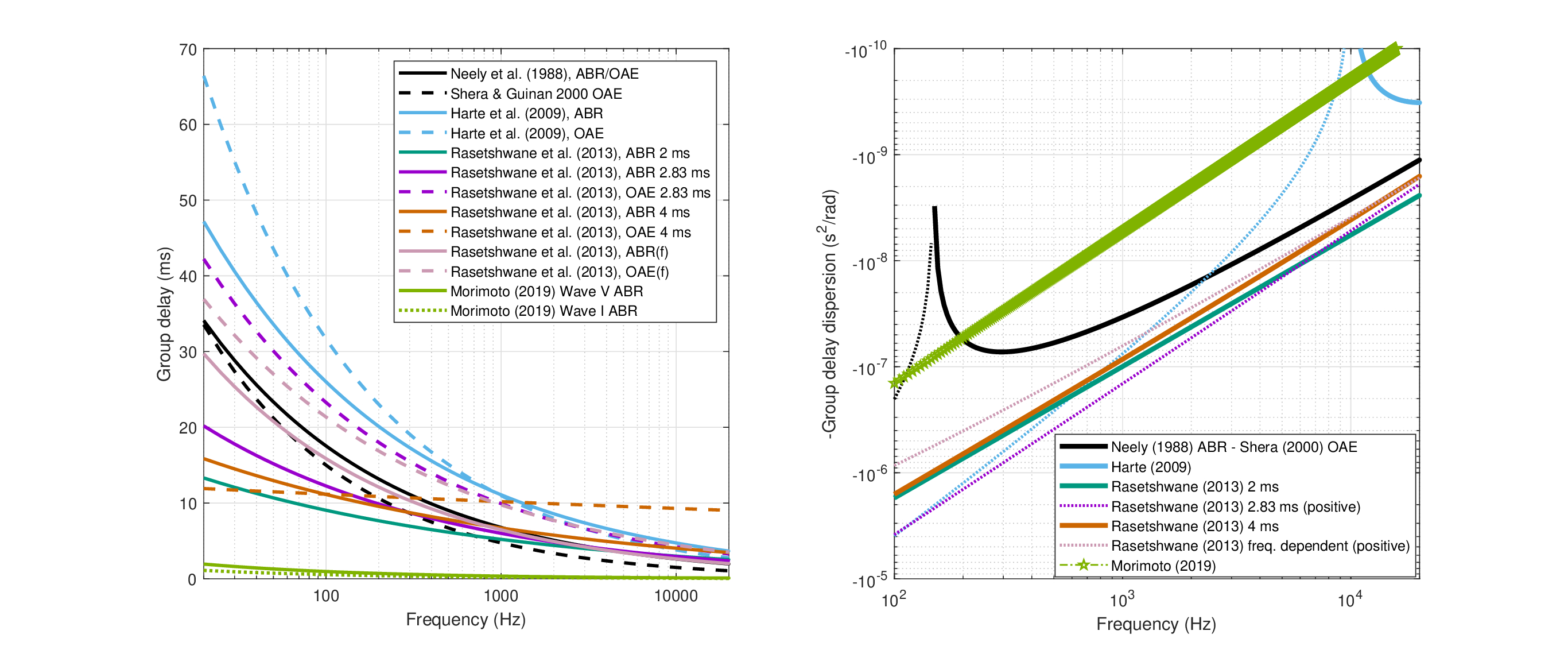
Figure 11.15: Neural group-delay dispersion estimates based on power-law fits from literature. Left: Cochlear (and neural) group delay fitted according to the power-law functions summarized in Table 11.1 (ABR—solid curves, OAE—dashed curves), omitting constant delays. Note that the curve for the 2 ms OAE condition of Rasetshwane et al. (2013) is identically 0 and does not appear on the plot. Two curves of frequency-dependent tone bursts are marked in the legend with (f). Right: The (negative) neural group-delay dispersion based on differences between the paired ABR and the OAE curves, which were taken as the neural group delay (Eq. 11.19). The dash-dot-star green curve marks the \(\tau_{gV} - \tau_{gI}\) dispersion according to Morimoto et al. (2019), which sets a lower bound for the complete neural dispersion path. Solid curves mark the (desired) negative dispersion, whereas dotted curves are positive.

Study	b	c	i	d	Level (dB SPL)	comments
Auditory brainstem response (ABR)
Neely et al. (1988)	12.9	5	L dB / 100 dB SPL	0.413	10–100	non-simultaneous ABR and OAE
Harte et al. (2009)	11.09	1	1	0.37	66	Tone burst ABR, 0.5–8 kHz
Rasetshwane et al. (2013, Table III)	9.99	5.1	L dB /100 dB	0.24	20–90	ABR, 2 ms tone bursts
11.47	5.05	L dB /100 dB	0.31	20–90	ABR, 2.83 ms tone bursts
13.89	6.17	L dB /100 dB	0.22	20–90	ABR, 4 ms tone bursts
12.63	5.34	L dB /100 dB	0.39	20–90	ABR, frequency-dependent tone bursts
Morimoto et al. (2019)	\(0.00920n_k/9\)	1	1	0.4356	60 dB HL, or 104 dB SPL (peak)	\(0\le n_k \le 9\), \(f\) in Hz and \(t_g\) in s; chirp ABR to find maximum wave-I response
Otoacoustic emissions (OAE)
Shera and Guinan Jr (2000)	0.15	1	1	0.5	40	OAE model was provided by Fobel and Dau (2004)
Harte et al. (2009)	10.98	1	1	0.46	66	Tone burst OAE, 0.5–8 kHz
Rasetshwane et al. (2013, Table V)	16.40	9.32	L dB /100 dB	0.00	20-90	OAE, 2 ms tone bursts
20.41	6.06	L dB /100 dB	0.37	20–90	ABR, 2.83 ms tone bursts
19.00	4.75	L dB /100 dB	0.04	20–90	ABR, 4 ms tone bursts
20.56	6.44	L dB /100 dB	0.34	20–90	ABR, frequency-dependent tone bursts

Table 11.1: Summary of various power-law fits found in literature for evoked otoacoustic emissions or auditory brainstem response data according to the power law prescribed by Neely et al. (1988), Eq. 11.20, where the frequency \(f\) is in kHz, and the group delay \(\tau_g\) in milliseconds. Wherever \(i \neq 1\), the fraction of the dB level \(L\) over 100 dB is used. Constant delays (e.g., 5 ms neural delay) are omitted. ABR level dependence of group delay that was observed to also be frequency dependent was modeled using a somewhat different power law in (Huang et al., 2022).

Since neural dispersion is currently a hypothetical property of the auditory system, the results from the study by Morimoto et al. (2019) were used to cross-validate it. The group delay of the chirps that were used as stimuli compensated for the neural group delay of the form given by Elberling and Don (2008) (“CE-chirp”):

\[ \tau_{g} = 0.00920\frac{n_k}{9} f^{-0.4356} \]

(11.21)

with the frequency \(f\) in Hz, and the integer parameter \(n_k\) varying between 0 and 9. By using chirps with the corresponding negative group delay, it was found that \(n_k=4\) maximized the wave-I response and \(n_k=7\) maximized the wave-V response. Thus, the same method as above can be used to estimate the group delay associated only with the wave-I to wave-V path, and differentiate it once to obtain the respective neural group dispersion:

\[ v_{V-I} = \frac{1}{2}\frac{d}{d\omega}(\tau_{gV} - \tau_{gI}) = \frac{-0.4356}{4\pi}0.00920\frac{7-4}{9} f^{-1.4356} = -0.0001063f^{-1.4356}\,\,\mathop{\mathrm{s}}^2 /\mathop{\mathrm{rad}} \]

(11.22)

Ideally, this partial group-delay dispersion (thick green curve in Figure 11.15, right) is smaller than the total path, \(|v_{V-I}|<|v|\), and has the same sign, which implies that the growth of the group-delay dispersion is a monotonic function of neural distance. This reasonable (yet unproven) assumption can be used as a key to select the negative group-delay dispersion results (solid curves in Figure 11.15), over the positive ones (dotted curves in Figure 11.15), which rules out the positive, frequency-dependent tone-burst measurements obtained by Harte et al. (2009) and Rasetshwane et al. (2013). Incidentally, the method in the latter responses was deemed invalid due to stimulus duration dependence (Ruggero and Temchin, 2007). Furthermore, the curve derived from Neely et al. (1988) and Shera and Guinan Jr (2000) is also positive at low frequencies and becomes smaller than the wave-V to wave-I data. This leaves the 2 and 4 ms fixed-rise-time responses by Rasetshwane et al. (2013) as the most favorable candidates from which to obtain the neural group-delay dispersion. However, for an unknown reason, the 2.83 ms fixed rise-time response Rasetshwane et al. (2013) did not produce the desired curve, which was expected to lie between the 2 and 4 ms curves. This discrepancy produces some uncertainty as for how confident we can be in the data using this method. However, as will turn out, the remaining 2 and 4 ms neural group dispersion data from Rasetshwane et al. (2013) both produced plausible values that could be employed in the rest of this work. Specifically, the 4 ms dataset produces slightly better results and was used throughout.

11.8 Discussion

This chapter systematically analyzed the dispersive properties of the human auditory path from the outer ear to the inferior colliculus (IC) in order to have plausible estimates of its group-delay dispersion. While the possibility of dispersion should not be controversial anywhere in the system, the segmentation process that leads to associating various elements in the system (summarized in Figure 11.1) with different measurements is not free of assumptions that may turn out to be inaccurate. Nowhere has it been more conspicuous than in and around the organ of Corti, wherein we hypothesized the time lens resides. As another layer of complexity, this work hypothesizes a mechanism for phase modulation that can neatly function as a time lens, but has not been explicitly measured to date. This adds up to the earlier theory that established a PLL function as yet another role for the OHCs. While the effect on the present data is inconsequential in many of the results obtained in the next chapters, at least some of these controversies will eventually have to be empirically settled in order to be able to get better estimates of the dispersive system parameters.

Several simplifying assumptions have been made to be able to parse the system more efficiently, which will have to be relaxed when higher certainty is obtained. The two main ones are the neglecting of all level considerations (data were obtained for low levels or 40 dB SPL, whenever possible) and the treatment of the entire audio range as scalable, with no regard for anomalies of low or high frequencies. Indeed, a correction will be required for frequencies below 500 Hz in some of the results obtained later. Another simplifying and necessary assumption has been to treat the different auditory pathways between the brainstem and the IC as a single dispersive path. We do not know whether the parallel processing of the brainstem is precisely timed, so that outputs from the two or three branches (VCN, DCN, PVCN) simultaneously converge in the IC, but two studies were mentioned that indicate that this may not be universally the case (Haplea et al., 1994; McGinley et al., 2012).

Neural transmission codes the information carried by the mechanical waves from the cochlea to the brain. As such, it was taken here as a proxy of a real physical process that has non-zero dispersion, by definition (see §3.4.2). Whether the dispersion itself is a feature of the auditory code or an epiphenomenon of its transmission is subject to future exploration. In this work, only the latter alternative is directly explored—dispersion that is evident from brainstem potentials that are not decoded, but are treated as aggregate activity that can be neurophysiologically localized.

An alternative derivation of the dispersion parameters will become possible at a much later stage of this work—once the full theory is developed—using a battery of four psychoacoustic tests (§F). With a limited pool of available data, most of the general trends observed above can be tentatively cross-validated, as long as the parameters are allowed to be complex, so absorption becomes more dominant. They suggest that at the lowest frequencies, one of the dispersion parameters—most likely the time-lens curvature—changes sign. However, this psychoacoustic solution is not going to be used in the text, as the majority of the studied effects can be studied qualitatively with the parameters obtained above, and without the troubling inclusion of absorption in the theory.

All in all, we obtained estimates for the cochlear and neural group-delay dispersions that turned out both negative. The time-lens curvature, in contrast, is positive. The combination of these three frequency-dependent parameters will be used to explore the temporal auditory imaging equations in the next chapters.

Footnotes

97. https://apps.automeris.io/wpd/ by Ankit Rohatgi.

98. If the point of the surface that is impacted by the wave does not interact with its vicinity, then the surface is said to be locally reactive. If the surface reacts as a whole (like a membrane), then its impedance is of extended reaction.

99. For example, see references to the cochlea as an “acoustic prism” in Shera et al. (2002), Oxenham (2014), and Altoè and Shera (2020).

100. The ABR and TOAE methods will be revisited in the section about neural dispersion §11.7, where these methods appear to have no alternatives, at present.

101. The live data refer to the active status of the OHCs, which provide frequency selectivity and compressive gain in normal listening conditions. In this work, the OHCs also have a role in time lensing, which is phase modulation in the time domain (§11.6). Hence, the effect of phase modulation can be thought to affect the cochlear group delay and group-delay dispersion figures from Ruggero and Temchin (2007). However, the nonlinear analysis in Temchin et al. (2005) and Ruggero and Temchin (2007) is based on Wiener-kernel method, which requires white noise as input to the nonlinear system. Typically, the system nonlinearity is considered static (time-invariant) (de Boer and de Jongh, 1978; van Dijk et al., 1994). However, there is nothing about the operation of the OHCs that suggests that it is static. While we do not know if the two functions are related, the amplificative OHC function could theoretically be almost instantaneous (Altoè et al., 2017), whereas the time lens operation may require buildup time to arrive to the operation point of its modulated stiffness (§11.6; see also §9.9.3). For such a system to work, the input has to be (partially) coherent, rather than totally incoherent (white noise). This means that the Wiener-kernel method may fail to engage the time-lens functionality of the OHCs and therefore may not disclose any phase modulation curvature. The exception may be at low frequencies, where the auditory narrowband filters can significantly cohere the input (§9.9.2). Of course, bypassing the time-lens is exactly what we would like to achieve in order to get a clean estimate of the cochlear dispersion.

102. But see a discussion about an apparent phase modulation in the chinchilla's BM basal response to clicks in Recio and Rhode (2000), where it was suggested that the modulation is a result of nonlinear and compressive processes and is likely not a mere artifact of BM motion.

103. The phase difference for a pure tone between the BM and the reticular lamina was recently measured in vivo in the gerbil (\(N=8\)) and presented in He and Ren (2021) in their Figure 4g and Supplementary Data 4. The two responses do not match, though, but both can be shown to have a small quadratic component once the linear phase component is removed from the CF region. In the case of the plotted response, the peak is above the CF and the curvature is an order of magnitude larger than in the spreadsheet data, which produce an almost negligible curvature that is part of faster broadband oscillation. Neither case is obviously consistent or inconsistent with the data from Dong and Olson (2013).

104. Because the linear term is usually very dominant, typical phase responses may appear completely linear, similar to a simple resonance of a bandpass filter. So curved components were removed from low-frequency auditory nerve responses in Allen (1983), which appear completely linear. In another more recent example, Lewis et al. (2002, Figure 6) used the Wiener-kernel technique to nonlinearly estimate the phase response from spike timing patterns in the auditory nerve, using a white noise input. However, no curvature information could be seen there, maybe due to the incoherent nature of the signal and the inability of the OHCs to phase lock to it.

105. While it is not attempted here to resolve it, a few provocative remarks should be made regarding the human frequency selectivity controversy. First, the very notion of a constant bandwidth that is fundamental in classical linear filters can be elusive in systems that exhibit suppression, emissions, feedback, level dependence, compression, and other nonlinear effects. The ongoing attempt to remove the confounding effects of these phenomena and obtain a reduced linear filter “kernel” may belie the generality and hence the usefulness of the concept of bandwidth, which drives this exploration in the first place, as each bandwidth applies only to a limited set of stimuli (see also, Thoret et al., 2023). Inasmuch as the PLL theory put forth in §9 may turn out to be correct, it will most certainty change the interpretation of some of the involved models (e.g, of OAEs and suppression) and their corresponding results. This is so because the PLL appears linear only when it is in lock and it has several bandwidths associated with different modes of operation (Figure §9.2). If we additionally consider a passive linear filter that precedes and “contains” the PLL, then some quasi-linear effects may be obtained that produce broad filtering, whereas under locked conditions, the filtering appear narrower. Combined with the filter sharpness controversy, the discussion about the correct place of filtering is reminiscent of the dreaded second filter problem, which suggested that there can be two stages of bandpass filtering in the cochlea. The problem was originally framed by Evans (1972) and Evans and Wilson (1973), who noted that the neural and mechanical data available at that time did not match. It has been considered more or less resolved ever since modern methods converged on very similar neural and mechanical results (Sellick et al., 1982; Khanna and Leonard, 1982). However, recent in-vivo measurements of vibrations within the organ of Corti have shown that the BM tuning is not as sharp as that recorded on the reticular lamina (Ren et al., 2016a), which may be interpreted to show the existence of a second filter after all. See Cooper et al. (2008) for a historical review and Bell (2005) for an alternative point of view. In order to keep the temporal imaging and PLL theories independent, we will leave the bandwidth interpretation question unanswered, at present.

106. This term has been used once in literature to analogize the function of the fish ear, but with no particular reasoning for why that is so (Yoda et al., 2002).

107. The chirp-evoked electrophysiological measurement was originally introduced by Shore and Nuttall (1985), in an attempt to counter the asynchronous auditory channel activation due to dispersion in click-evoked compound action potential measurement. The underlying principle here is essentially the same as chirp radars and ultrashort pulse generation, where inverse operations are used to compress otherwise long pulses whose power is too dispersed (§10.1).

108. Note that the IC itself does not produce strong enough electric field that can be detected with ABR due to its disorganized layout. Hence, wave V corresponds to an earlier timing than would characterize the central nucleus of the IC—usually attributed to the area between the LL and the IC (Hall III, 2007; p. 45–46).

109. Recent recordings of the octopus cells in gerbils uncovered high temporal precision that is also sensitive to the direction of linear frequency sweeps around frequency “hot spots” (i.e., tuned input fibers from the auditory nerve)—a cellular detection mechanism that appears to be independent of the coincidence detection mechanism (Lu et al., 2022).

110. Note that the group delay level dependence itself appears to be frequency dependent, as was recently shown for ABR measurements by Huang et al. (2022).

111. Other ABR and OAE estimates that were not necessarily fitted by power laws were compiled in Moleti and Sisto (2008), but were not explored here.

References

Aibara, Ryuichi, Welsh, Joseph T, Puria, Sunil, and Goode, Richard L. Human middle-ear sound transfer function and cochlear input impedance. Hearing Research, 152 (1): 100–109, 2001.

Aitkin, Lindsay M and Phillips, Stephen C. Is the inferior colliculus and obligatory relay in the cat auditory system? Neuroscience Letters, 44 (3): 259–264, 1984.

Allen, Jont B. Magnitude and phase-frequency response to single tones in the auditory nerve. The Journal of the Acoustical Society of America, 73 (6): 2071–2092, 1983.

Altoè, Alessandro, Charaziak, Karolina K, and Shera, Christopher A. Dynamics of cochlear nonlinearity: Automatic gain control or instantaneous damping? The Journal of the Acoustical Society of America, 142 (6): 3510–3519, 2017.

Altoè, Alessandro and Shera, Christopher A. The cochlear ear horn: Geometric origin of tonotopic variations in auditory signal processing. Scientific Reports, 10 (1): 1–10, 2020.

Anderson, David J, Rose, Jerzy E, Hind, Joseph E, and Brugge, John F. Temporal position of discharges in single auditory nerve fibers within the cycle of a sine-wave stimulus: Frequency and intensity effects. The Journal of the Acoustical Society of America, 49 (4B): 1131–1139, 1971.

Ashmore, Jonathan. Cochlear outer hair cell motility. Physiological Reviews, 88 (1): 173–210, 2008.

Azhari, Haim. Basics of Biomedical Ultrasound for Engineers. John Wiley & Sons, 2010.

Babahosseini, Hesam, Belyantseva, Inna A., Yousaf, Rizwan, Tona, Risa, Hadi, Shadan, Inagaki, Sayaka, Wilson, Elizabeth, Kitajiri, Shin-ichiro, Frolenkov, Gregory I., Friedman, Thomas B., and Cartagena-Rivera, Alexander X. Unbalanced bidirectional radial stiffness gradients within the organ of Corti promoted by TRIOBP. Proceedings of the National Academy of Sciences, 119: e2115190119, 2022.

Bass, Andrew H, Rose, Gary J, and Pritz, Michael B. Auditory midbrain of fish, amphibians, and reptiles: Model systems for understanding auditory function. In Winer, Jeffery A. and Schreiner, Christoph E., editors, The Inferior Colliculus, pages 459–492. Springer Science+Business Media, Inc., 2005.

Békésy, Georg von. On the elasticity of the cochlear partition. The Journal of the Acoustical Society of America, 20 (3): 227–241, 1948.

Békésy, Georg von. On the resonance curve and the decay period at various points on the cochlear partition. The Journal of the Acoustical Society of America, 21 (3): 245–254, 1943/1949. Originally appeared as “Über die Resonanzkurve und die Abklifigzeit der verschiedenen Stellen der Schneckentrennwand,” Akustische Zeits. 8, 66–76 (1943).

Békésy, Georg von. Experiments in Hearing. McGraw-Hill Book Company, Inc., 1960. translated by E. G. Wever.

Bell, James Andrew. The Underwater Piano: A Resonance Theory of Cochlear Mechanics. PhD thesis, The Australian National University, 2005.

Bell, Andrew. A resonance approach to cochlear mechanics. PloS One, 7 (11): e47918, 2012a.

Bell, Andrew. Reptile ears and mammalian ears: Hearing without a travelling wave. Journal of Hearing Science, 2 (3): 14–22, 2012b.

Blauert, Jens. Spatial Hearing: The Psychophysics of Human Sound Localization. MIT press, Cambridge, MA, revised edition edition, 1997.

Brass, David and Locke, Antony. The effect of the evanescent wave upon acoustic measurements in the human ear canal. The Journal of the Acoustical Society of America, 101 (4): 2164–2175, 1997.

Brillouin, Léon. Wave Propagation and Group Velocity. Academic Press, Inc., 1960.

Burton, Jane A, Dylla, Margit E, and Ramachandran, Ramnarayan. Frequency selectivity in macaque monkeys measured using a notched-noise method. Hearing Research, 357: 73–80, 2018.

Caldwell, Marc, Souza, Pamela E, and Tremblay, Kelly L. Effect of probe tube insertion depth on spectral measures of speech. Trends in Amplification, 10 (3): 145–154, 2006.

Carney, Laurel H, McDuffy, Megean J, and Shekhter, Ilya. Frequency glides in the impulse responses of auditory-nerve fibers. The Journal of the Acoustical Society of America, 105 (4): 2384–2391, 1999.

Casseday, JH and Covey, E. A neuroethological theory of the operation of the inferior colliculus. Brain, Behavior and Evolution, 47 (6): 323–336, 1996.

Charman, Neil. Optics of the eye. In Bass, Michael, Enoch, Jay M., and Lakshminarayanan, Vasudevan, editors, Handbook of Optics. Fundamentals, Techniques, & Design, volume 3, pages 1.1–1.65. McGraw-Hill Companies Inc., 2nd edition, 2010.

Chen, Fangyi, Zha, Dingjun, Fridberger, Anders, Zheng, Jiefu, Choudhury, Niloy, Jacques, Steven L, Wang, Ruikang K, Shi, Xiaorui, and Nuttall, Alfred L. A differentially amplified motion in the ear for near-threshold sound detection. Nature Neuroscience, 14 (6): 770, 2011.

Cheng, Jeffrey Tao, Hamade, Mohamad, Merchant, Saumil N, Rosowski, John J, Harrington, Ellery, and Furlong, Cosme. Wave motion on the surface of the human tympanic membrane: Holographic measurement and modeling analysis. The Journal of the Acoustical Society of America, 133 (2): 918–937, 2013.

Cooper, N and Shera, C. Backward-traveling waves in the cochlea (poster). In Association for Research in Otolaryngology Twenty-seventh Midwinter Research Meeting; Daytona Beach, Florida, page 342, 2004.

Cooper, Nigel P, Pickles, James O Pickles, and Manley, Geoffrey A. Traveling waves, second filters, and physiological vulnerability: A short history of the discovery of active processes in hearing. In Manley, Geoffrey A, Fay, Richard R, and Popper, Arthur N, editors, Active processes and otoacoustic emissions in hearing, volume 30, pages 39–62. Springer Science & Business Media, LLC, New York, NY, 2008.

Cooper, Nigel P, Vavakou, Anna, and van der Heijden, Marcel. Vibration hotspots reveal longitudinal funneling of sound-evoked motion in the mammalian cochlea. Nature Communications, 9 (1): 1–12, 2018.

Cooper, Nigel P and van der Heijden, Marcel. Dynamics of cochlear nonlinearity. In van Dijk, Pim, Başkent, Deniz, Gaudrain, Etienne, de Kleine, Emile, Wagner, Anita, and Lanting, Cris, editors, Physiology, Psychoacoustics and Cognition in Normal and Impaired Hearing, pages 267–274. Springer International Publishing AG, Cham, Switzerland, 2016.

Dallos, Peter, Wu, Xudong, Cheatham, Mary Ann, Gao, Jiangang, Zheng, Jing, Anderson, Charles T, Jia, Shuping, Wang, Xiang, Cheng, Wendy HY, Sengupta, Soma, He, David Z.Z., and Zuo, Jian. Prestin-based outer hair cell motility is necessary for mammalian cochlear amplification. Neuron, 58 (3): 333–339, 2008.

Davis, Hallowell. A model for transducer action in the cochlea. In Cold Spring Harbor Symposia on Quantitative Biology, volume 30, pages 181–190. Cold Spring Harbor Laboratory Press, 1965.

Dewey, James B, Altoè, Alessandro, Shera, Christopher A, Applegate, Brian E, and Oghalai, John S. Cochlear outer hair cell electromotility enhances organ of Corti motion on a cycle-by-cycle basis at high frequencies in vivo. Proceedings of the National Academy of Sciences, 118 (43), 2021.

Don, Manuel and Eggermont, JJ. Analysis of the click-evoked brainstem potentials in man using high-pass noise masking. The journal of the acoustical society of America, 63 (4): 1084–1092, 1978.

Dong, Wei and Olson, Elizabeth S. Detection of cochlear amplification and its activation. Biophysical journal, 105 (4): 1067–1078, 2013.

Duifhuis, Hendrikus. Cochlear Mechanics: Introduction to a Time Domain Analysis of the Nonlinear Cochlea. Springer Science & Business Media, New York, NY, 2012.

Elberling, Claus and Don, Manuel. Auditory brainstem responses to a chirp stimulus designed from derived-band latencies in normal-hearing subjects. The Journal of the Acoustical Society of America, 124 (5): 3022–3037, 2008.

Elberling, Claus and Don, Manuel. A direct approach for the design of chirp stimuli used for the recording of auditory brainstem responses. The Journal of the Acoustical Society of America, 128 (5): 2955–2964, 2010.

Elliott, Stephen J, Ni, Guangjian, Mace, Brian R, and Lineton, Ben. A wave finite element analysis of the passive cochlea. The Journal of the Acoustical Society of America, 133 (3): 1535–1545, 2013.

Emadi, Gulam, Richter, Claus-Peter, and Dallos, Peter. Stiffness of the gerbil basilar membrane: Radial and longitudinal variations. Journal of neurophysiology, 91 (1): 474–488, 2004.

Evans, EF. The frequency response and other properties of single fibres in the guinea-pig cochlear nerve. The Journal of Physiology, 226 (1): 263–287, 1972.

Evans, E. F and Wilson, J. P. The frequency selectivity of the cochlea. In Mø ller, Aage R. and Boston, Pamela, editors, Basic Mechanisms in Hearing, pages 519–554. Academic Press Inc., New York and London, 1973.

Fallah, Elika, Strimbu, C Elliott, and Olson, Elizabeth S. Nonlinearity of intracochlear motion and local cochlear microphonic: Comparison between guinea pig and gerbil. Hearing Research, page 108234, 2021.

Farrahi, Shirin, Ghaffari, Roozbeh, Sellon, Jonathan B, Nakajima, Hideko H, and Freeman, Dennis M. Tectorial membrane traveling waves underlie sharp auditory tuning in humans. Biophysical Journal, 111 (5): 921–924, 2016.

Fay, Jonathan P, Puria, Sunil, and Steele, Charles R. The discordant eardrum. Proceedings of the National Academy of Sciences, 103 (52): 19743–19748, 2006.

Fletcher, Neville H and Rossing, Thomas D. The physics of musical instruments. Springer Science+Business Media New York, 2nd edition, 1998.

Fobel, Oliver and Dau, Torsten. Searching for the optimal stimulus eliciting auditory brainstem responses in humans. The Journal of the Acoustical Society of America, 116 (4): 2213–2222, 2004.

Geisler, C Daniel and Rhode, William S. The phases of basilar-membrane vibrations. The Journal of the Acoustical Society of America, 71 (5): 1201–1203, 1982.

Glasberg, Brian R and Moore, Brian CJ. Derivation of auditory filter shapes from notched-noise data. Hearing Research, 47 (1-2): 103–138, 1990.

Goode, Richard L, Friedrichs, Robert, and Falk, Stephen. Effect on hearing thresholds of surgical modification of the external ear. Annals of Otology, Rhinology & Laryngology, 86 (4): 441–450, 1977.

Gorga, Michael P, Kaminski, Jan R, Beauchaine, Kathryn A, and Jesteadt, Walt. Auditory brainstem responses to tone bursts in normally hearing subjects. Journal of Speech, Language, and Hearing Research, 31 (1): 87–97, 1988.

Greenwood, Donald D. A cochlear frequency-position function for several species"”29 years later. The Journal of the Acoustical Society of America, 87 (6): 2592–2605, 1990.

Guinan Jr, John J and Cooper, Nigel P. Medial olivocochlear efferent inhibition of basilar-membrane responses to clicks: Evidence for two modes of cochlear mechanical excitation. The Journal of the Acoustical Society of America, 124 (2): 1080–1092, 2008.

Hall III, James W. New Handbook of Auditory Evoked Responses. Pearson Education, Inc., Boston, MA, 2007.

Hallworth, Richard. Absence of voltage-dependent compliance in high-frequency cochlear outer hair cells. Journal of the Association for Research in Otolaryngology, 8 (4): 464–473, 2007.

Haplea, S, Covey, E, and Casseday, JH. Frequency tuning and response latencies at three levels in the brainstem of the echolocating bat, Eptesicus fuscus. Journal of Comparative Physiology A, 174 (6): 671–683, 1994.

Harte, James M, Pigasse, Gilles, and Dau, Torsten. Comparison of cochlear delay estimates using otoacoustic emissions and auditory brainstem responses. The Journal of the Acoustical Society of America, 126 (3): 1291–1301, 2009.

Hashimoto, I. Auditory evoked potentials from the human midbrain: Slow brain stem responses. Electroencephalography and Clinical Neurophysiology, 53 (6): 652–657, 1982.

He, David ZZ and Dallos, Peter. Somatic stiffness of cochlear outer hair cells is voltage-dependent. Proceedings of the National Academy of Sciences, 96 (14): 8223–8228, 1999.

He, Wenxuan and Ren, Tianying. Basilar membrane vibration is not involved in the reverse propagation of otoacoustic emissions. Scientific Reports, 3: 1874, 2013.

He, Wenxuan, Fridberger, Anders, Porsov, Edward, Grosh, Karl, and Ren, Tianying. Reverse wave propagation in the cochlea. Proceedings of the National Academy of Sciences, 105 (7): 2729–2733, 2008b.

He, Wenxuan and Ren, Tianying. The origin of mechanical harmonic distortion within the organ of corti in living gerbil cochleae. Communications Biology, 4 (1): 1–11, 2021.

van der Heijden, Marcel and Versteegh, Corstiaen PC. Energy flux in the cochlea: Evidence against power amplification of the traveling wave. Journal of the Association for Research in Otolaryngology, 16 (5): 581–597, 2015a.

Homma, Kenji, Du, Yu, Shimizu, Yoshitaka, and Puria, Sunil. Ossicular resonance modes of the human middle ear for bone and air conduction. The Journal of the Acoustical Society of America, 125 (2): 968–979, 2009.

Huang, Hsuan, Chen, Yu-Fu, Hsu, Chien-Yeh, Cheng, Yen-Fu, and Yang, Tzong-Hann. Evaluating auditory brainstem response to a level-dependent chirp designed based on derived-band latencies. The Journal of the Acoustical Society of America, 151 (4): 2688–2700, 2022.

Hudde, HASS and Schmidt, S. Sound fields in generally shaped curved ear canals. The Journal of the Acoustical Society of America, 125 (5): 3146–3157, 2009.

Joris, PX, Schreiner, CE, and Rees, A. Neural processing of amplitude-modulated sounds. Physiological Reviews, 84 (2): 541–577, 2004.

Joris, Philip X, Bergevin, Christopher, Kalluri, Radha, Mc Laughlin, Myles, Michelet, Pascal, van der Heijden, Marcel, and Shera, Christopher A. Frequency selectivity in old-world monkeys corroborates sharp cochlear tuning in humans. Proceedings of the National Academy of Sciences, 108 (42): 17516–17520, 2011.

Keefe, Douglas H, Bulen, Jay C, Arehart, Kathy Hoberg, and Burns, Edward M. Ear-canal impedance and reflection coefficient in human infants and adults. The Journal of the Acoustical Society of America, 94 (5): 2617–2638, 1993.

Kemp, David T. Stimulated acoustic emissions from within the human auditory system. The Journal of the Acoustical Society of America, 64 (5): 1386–1391, 1978.

Kemp, David T. Otoacoustic emissions: Concepts and origins. In Manley, Geoffrey A, Fay, Richard R, and Popper, Arthur N, editors, Active Processes and Otoacoustic Emissions in Hearing, volume 30, pages 1–38. Springer Science & Business Media, LLC, New York, NY, 2007.

Kennedy, C., Sakurada, O., Shinohara, M., Jehle, J., and Sokoloff, L. Local cerebral glucose utilization in the normal conscious macaque monkey. Annals of Neurology, 4 (4): 293–301, 1978.

Khanna, SM and Stinson, Michael R. Specification of the acoustical input to the ear at high frequencies. The Journal of the Acoustical Society of America, 77 (2): 577–589, 1985.

Khanna, Shyam M and Leonard, Debra GB. Basilar membrane tuning in the cat cochlea. Science, 215 (4530): 305–306, 1982.

Kinsler, Lawrence E, Frey, Austin R, Coppens, Alan B, and Sanders, James V. Fundamentals of Acoustics. John Wiley & Sons, Inc., New York, NY, 4th edition, 1999.

Kittel, Malte, Wagner, Eva, and Klump, Georg M. An estimate of the auditory-filter bandwidth in the Mongolian gerbil. Hearing Research, 164 (1-2): 69–76, 2002.

Kohlrausch, Armin and Sander, Andres. Phase effects in masking related to dispersion in the inner ear. II. Masking period patterns of short targets. The Journal of the Acoustical Society of America, 97 (3): 1817–1829, 1995.

Kolner, Brian H. Space-time duality and the theory of temporal imaging. IEEE Journal of Quantum Electronics, 30 (8): 1951–1963, 1994a.

Kolner, Brian H. Generalization of the concepts of focal length and f-number to space and time. The Journal of the Optical Society of America A, 11 (12): 3229–3234, 1994b.

Kraus, Nina, Smith, D Ian, McGee, Therese, Stein, Laszlo, and Cartee, Cheryl. Development of the middle latency response in an animal model and its relation to the human response. Hearing Research, 27 (2): 165–176, 1987.

Kudo, Motoi and Niimi, Kahee. Ascending projections of the inferior colliculus in the cat: An autoradiographic study. Journal of Comparative Neurology, 191 (4): 545–556, 1980.

Kulesza Jr, Randy J, Viñuela, Antonio, Saldaña, Enrique, and Berrebi, Albert S. Unbiased stereological estimates of neuron number in subcortical auditory nuclei of the rat. Hearing Research, 168 (1–2): 12–24, 2002.

Kvale, Mark N and Schreiner, Christoph E. Short-term adaptation of auditory receptive fields to dynamic stimuli. Journal of Neurophysiology, 91 (2): 604–612, 2004.

Langner, Gerald. Neural processing and representation of periodicity pitch. Acta Oto-Laryngologica, 117 (sup532): 68–76, 1997.

Lewis, Edwin R, Henry, Kenneth R, and Yamada, Walter M. Tuning and timing in the gerbil ear: Wiener-kernel analysis. Hearing Research, 174 (1-2): 206–221, 2002.

Liberman, M Charles. Auditory-nerve response from cats raised in a low-noise chamber. The Journal of the Acoustical Society of America, 63 (2): 442–455, 1978.

Lighthill, James. Energy flow in the cochlea. Journal of Fluid Mechanics, 106: 149–213, 1981.

Lin, Tai and Guinan Jr, John J. Time–frequency analysis of auditory-nerve-fiber and basilar-membrane click responses reveal glide irregularities and non-characteristic-frequency skirts. The Journal of the Acoustical Society of America, 116 (1): 405–416, 2004.

Liu, Yi-Wen and Neely, Stephen T. Outer hair cell electromechanical properties in a nonlinear piezoelectric model. The Journal of the Acoustical Society of America, 126 (2): 751–761, 2009.

Lopez-Poveda, Enrique A and Eustaquio-Martin, Almudena. On the controversy about the sharpness of human cochlear tuning. Journal of the Association for Research in Otolaryngology, 14 (5): 673–686, 2013a.

Lu, Hsin-Wei, Smith, Philip H, and Joris, Philip X. Mammalian octopus cells are direction selective to frequency sweeps by excitatory synaptic sequence detection. Proceedings of the National Academy of Sciences, 119 (44): e2203748119, 2022.

Malmierca, Manuel S. and Hackett, Troy A. Structural organization of the ascending auditory pathway. In Rees, Adrian and Palmer, Alan R, editors, The Oxford Handbook of Auditory Science: The Auditory Brain, volume 2, pages 9–41. Oxford university press, New York, USA, 2010.

Manley, Geoffrey A, Köppl, Christine, and Bergevin, Christopher. Common substructure in otoacoustic emission spectra of land vertebrates. In AIP Conference Proceedings, 1703, pages 090012–1–090012–5. AIP Publishing LLC, 2015.

Manley, Geoffrey A and van Dijk, Pim. Frequency selectivity of the human cochlea: Suppression tuning of spontaneous otoacoustic emissions. Hearing Research, 336: 53–62, 2016.

Eustaquio-Martín, Almudena and Lopez-Poveda, Enrique A. Isoresponse versus isoinput estimates of cochlear filter tuning. Journal of the Association for Research in Otolaryngology, 12 (3): 281–299, 2011.

McGee, Therese, Kraus, Nina, Comperatore, Carlos, and Nicol, Trent. Subcortical and cortical components of the MLR generating system. Brain Research, 544 (2): 211–220, 1991.

McGinley, Matthew J, Liberman, M Charles, Bal, Ramazan, and Oertel, Donata. Generating synchrony from the asynchronous: Compensation for cochlear traveling wave delays by the dendrites of individual brainstem neurons. Journal of Neuroscience, 32 (27): 9301–9311, 2012.

Meenderink, Sebastiaan WF and Dong, Wei. Organ of Corti vibrations are dominated by longitudinal motion in vivo. Communications Biology, 5 (1): 1285, 2022.

Mehrgardt, Sünke and Mellert, Volker. Transformation characteristics of the external human ear. The Journal of the Acoustical Society of America, 61 (6): 1567–1576, 1977.

Moleti, Arturo and Sisto, Renata. Comparison between otoacoustic and auditory brainstem response latencies supports slow backward propagation of otoacoustic emissions. The Journal of the Acoustical Society of America, 123 (3): 1495–1503, 2008.

Møller, Aage R. Coding of sounds with rapidly varying spectrum in the cochlear nucleus. The Journal of the Acoustical Society of America, 55 (3): 631–640, 1974.

Morimoto, Takashi, Fujisaka, Yoh-ichi, Okamoto, Yasuhide, and Irino, Toshio. Rising-frequency chirp stimulus to effectively enhance wave-I amplitude of auditory brainstem response. Hearing Research, 377: 104–108, 2019.

Morse, Philip M. and Ingard, K. Uno. Theoretical Acoustics. Princeton University Press, Princeton, NJ, 1968.

Müller, Marcus. The cochlear place-frequency map of the adult and developing Mongolian gerbil. Hearing Research, 94 (1-2): 148–156, 1996.

Musiek, Frank and Nagle, Stephanie. The middle latency response: A review of findings in various central nervous system lesions. Journal of the American Academy of Audiology, 29 (09): 855–867, 2018.

Naidu, Ram C and Mountain, David C. Measurements of the stiffness map challenge a basic tenet of cochlear theories. Hearing Research, 124 (1-2): 124–131, 1998.

Nakajima, Hideko Heidi, Dong, Wei, Olson, Elizabeth S, Merchant, Saumil N, Ravicz, Michael E, and Rosowski, John J. Differential intracochlear sound pressure measurements in normal human temporal bones. Journal of the Association for Research in Otolaryngology, 10 (1): 23, 2009.

Neely, ST, Norton, SJ, Gorga, MP, and Jesteadt, W. Latency of auditory brain-stem responses and otoacoustic emissions using tone-burst stimuli. The Journal of the Acoustical Society of America, 83 (2): 652–656, 1988.

Norton, Susan J and Neely, Stephen T. Tone-burst-evoked otoacoustic emissions from normal-hearing subjects. The Journal of the Acoustical Society of America, 81 (6): 1860–1872, 1987.

Nuttall, Alfred L, Ricci, Anthony J, Burwood, George, Harte, James M, Stenfelt, Stefan, Cayé-Thomasen, Per, Ren, Tianying, Ramamoorthy, Sripriya, Zhang, Yuan, Wilson, Teresa, Lunner, Thomas, Moore, Brian C. J., and Fridberger, Anders. A mechanoelectrical mechanism for detection of sound envelopes in the hearing organ. Nature Communications, 9 (1): 1–11, 2018.

Oxenham, Andrew J. Masking and masking release. In Jaeger, Dieter and Jung, Ranu, editors, Encyclopedia of Computational Neuroscience, pages 1661–1662. Springer New York, New York, NY, 2014.

Oxenham, Andrew J and Dau, Torsten. Towards a measure of auditory-filter phase response. The Journal of the Acoustical Society of America, 110 (6): 3169–3178, 2001a.

Oxenham, Andrew J and Dau, Torsten. Reconciling frequency selectivity and phase effects in masking. The Journal of the Acoustical Society of America, 110 (3): 1525–1538, 2001b.

Oxenham, Andrew J and Shera, Christopher A. Estimates of human cochlear tuning at low levels using forward and simultaneous masking. Journal of the Association for Research in Otolaryngology, 4 (4): 541–554, 2003.

Palmer, AR and Russell, IJ. Phase-locking in the cochlear nerve of the guinea-pig and its relation to the receptor potential of inner hair-cells. Hearing Research, 24 (1): 1–15, 1986.

Palmer, Alan R and Shackleton, Trevor M. Variation in the phase of response to low-frequency pure tones in the guinea pig auditory nerve as functions of stimulus level and frequency. Journal of the Association for Research in Otolaryngology, 10 (2): 233–250, 2009.

Perkel, Donald H and Bullock, Theodore H. Neural coding. Neurosciences Research Program Bulletin, 6 (3): 221–348, 1968.

Peterson, LC and Bogert, BP. A dynamical theory of the cochlea. The Journal of the Acoustical Society of America, 22 (3): 369–381, 1950.

Picton, Terry W, Hillyard, Steven A, Krausz, Howard I, and Galambos, Robert. Human auditory evoked potentials. I: Evaluation of components. Electroencephalography and Clinical Neurophysiology, 36: 179–190, 1974.

Probst, Rudolf, Lonsbury-Martin, Brenda L, and Martin, Glen K. A review of otoacoustic emissions. The Journal of the Acoustical Society of America, 89 (5): 2027–2067, 1991.

Puria, Sunil and Allen, Jont B. Measurements and model of the cat middle ear: Evidence of tympanic membrane acoustic delay. The Journal of the Acoustical Society of America, 104 (6): 3463–3481, 1998.

Puria, Sunil and Steele, Charles. Tympanic-membrane and malleus–incus-complex co-adaptations for high-frequency hearing in mammals. Hearing Research, 263 (1-2): 183–190, 2010.

Rabbitt, RD and Holmes, MH. Three-dimensional acoustic waves in the ear canal and their interaction with the tympanic membrane. The Journal of the Acoustical Society of America, 83 (3): 1064–1080, 1988.

Rabbitt, RD and Friedrich, MT. Ear canal cross-sectional pressure distributions: Mathematical analysis and computation. The Journal of the Acoustical Society of America, 89 (5): 2379–2390, 1991.

Ramamoorthy, Sripriya, Zha, Ding-Jun, and Nuttall, Alfred L. The biophysical origin of traveling-wave dispersion in the cochlea. Biophysical Journal, 99 (6): 1687–1695, 2010.

Rasetshwane, Daniel M, Argenyi, Michael, Neely, Stephen T, Kopun, Judy G, and Gorga, Michael P. Latency of tone-burst-evoked auditory brain stem responses and otoacoustic emissions: Level, frequency, and rise-time effects. The Journal of the Acoustical Society of America, 133 (5): 2803–2817, 2013.

Rasetshwane, Daniel M and Neely, Stephen T. Inverse solution of ear-canal area function from reflectance. The Journal of the Acoustical Society of America, 130 (6): 3873–3881, 2011.

Rea, Paul. Clinical Anatomy of the Cranial Nerves. Academic Press, Elsevier Inc., London, UK, 2014.

Recio, Alberto, Rich, Nola C, Narayan, S Shyamla, and Ruggero, Mario A. Basilar-membrane responses to clicks at the base of the chinchilla cochlea. The Journal of the Acoustical Society of America, 103 (4): 1972–1989, 1998.

Recio, Alberto and Rhode, William S. Basilar membrane responses to broadband stimuli. The Journal of the Acoustical Society of America, 108 (5): 2281–2298, 2000.

Recio-Spinoso, Alberto, Temchin, Andrei N, van Dijk, Pim, Fan, Yun-Hui, and Ruggero, Mario A. Wiener-kernel analysis of responses to noise of chinchilla auditory-nerve fibers. Journal of neurophysiology, 93 (6): 3615–3634, 2005.

Recio-Spinoso, Alberto and Rhode, William S. Fast waves at the base of the cochlea. PloS One, 10 (6): e0129556, 2015.

Ren, Tianying. Longitudinal pattern of basilar membrane vibration in the sensitive cochlea. Proceedings of the National Academy of Sciences, 99 (26): 17101–17106, 2002.

Ren, Tianying, He, Wenxuan, and Kemp, David. Reticular lamina and basilar membrane vibrations in living mouse cochleae. Proceedings of the National Academy of Sciences, 113 (35): 9910–9915, 2016b.

Ren, Tianying, He, Wenxuan, and Barr-Gillespie, Peter G. Reverse transduction measured in the living cochlea by low-coherence heterodyne interferometry. Nature Communications, 7 (1): 1–9, 2016a.

Rhode, William S. Observations of the vibration of the basilar membrane in squirrel monkeys using the mössbauer technique. The Journal of the Acoustical Society of America, 49 (4B): 1218–1231, 1971.

Robles, Luis and Ruggero, Mario A. Mechanics of the mammalian cochlea. Physiological Reviews, 81 (3): 1305–1352, 2001.

de La Rochefoucauld, Ombeline and Olson, Elizabeth S. The role of organ of Corti mass in passive cochlear tuning. Biophysical Journal, 93 (10): 3434–3450, 2007.

Rosowski, John J. Outer and middle ears. In Popper, Arthur N and Fay, Richard R, editors, Comparative Hearing: Mammals, volume 4, pages 172–247. Springer-Verlag New York Inc., 1994.

Rosowski, John J, Ramier, Antoine, Cheng, Jeffrey Tao, and Yun, Seok-Hyun. Optical coherence tomographic measurements of the sound-induced motion of the ossicular chain in chinchillas: Additional modes of ossicular motion enhance the mechanical response of the chinchilla middle ear at higher frequencies. Hearing Research, 396: 108056, 2020.

Ruggero, Mario A and Rich, Nola C. Timing of spike initiation in cochlear afferents: Dependence on site of innervation. Journal of Neurophysiology, 58 (2): 379–403, 1987.

Ruggero, Mario A, Rich, Nola C, Recio, Alberto, Narayan, S Shyamla, and Robles, Luis. Basilar-membrane responses to tones at the base of the chinchilla cochlea. The Journal of the Acoustical Society of America, 101 (4): 2151–2163, 1997.

Ruggero, Mario A and Temchin, Andrei N. Unexceptional sharpness of frequency tuning in the human cochlea. Proceedings of the National Academy of Sciences, 102 (51): 18614–18619, 2005.

Ruggero, Mario A and Temchin, Andrei N. Similarity of traveling-wave delays in the hearing organs of humans and other tetrapods. Journal for the Association for Research in Otolaryngology, 8 (2): 153–166, 2007.

Saremi, Amin, Beutelmann, Rainer, Dietz, Mathias, Ashida, Go, Kretzberg, Jutta, and Verhulst, Sarah. A comparative study of seven human cochlear filter models. The Journal of the Acoustical Society of America, 140 (3): 1618–1634, 2016.

Scherer, Marc P and Gummer, Anthony W. Impedance analysis of the organ of Corti with magnetically actuated probes. Biophysical Journal, 87 (2): 1378–1391, 2004.

Sellick, PM, Patuzzi, RMJB, and Johnstone, BM. Measurement of basilar membrane motion in the guinea pig using the mössbauer technique. The Journal of the Acoustical Society of America, 72 (1): 131–141, 1982.

Shen, Yi and Lentz, Jennifer J. Level dependence in behavioral measurements of auditory-filter phase characteristics. The Journal of the Acoustical Society of America, 126 (5): 2501–2510, 2009.

Shera, Christopher A, Guinan, John J, and Oxenham, Andrew J. Revised estimates of human cochlear tuning from otoacoustic and behavioral measurements. Proceedings of the National Academy of Sciences, 99 (5): 3318–3323, 2002.

Shera, Christopher A and Guinan Jr, John J. Stimulus-frequency-emission group delay: A test of coherent reflection filtering and a window on cochlear tuning. The Journal of the Acoustical Society of America, 113 (5): 2762–2772, 2003.

Shera, Christopher A. and Guinan Jr., John J. Mechanisms of mammalian otoacoustic emission. In Manley, Geoffrey A, Fay, Richard R, and Popper, Arthur N, editors, Active Processes and Otoacoustic Emissions in Hearing, volume 30, pages 305–342. Springer Science & Business Media, LLC, New York, NY, 2008.

Shera, Christopher A, Guinan, John J, and Oxenham, Andrew J. Otoacoustic estimation of cochlear tuning: Validation in the chinchilla. Journal of the Association for Research in Otolaryngology, 11 (3): 343–365, 2010.

Shera, Christopher A and Cooper, Nigel P. Basilar-membrane interference patterns from multiple internal reflection of cochlear traveling waves. The Journal of the Acoustical Society of America, 133 (4): 2224–2239, 2013.

Shera, Christopher A. Iterated intracochlear reflection shapes the envelopes of basilar-membrane click responses. The Journal of the Acoustical Society of America, 138 (6): 3717–3722, 2015.

Shera, Christopher A and Guinan Jr, John J. Frequency dependence of stimulus-frequency-emission phase: Implications for cochlear mechanics. In Wada, H., Takasaka, T., Ikeda, K., Ohyama, K., and Koike, T., editors, Recent Developments In Auditory Mechanics, pages 381–387. World Scientific, Singapore, 2000.

Shofner, William P, Sparks, Kathryn, Wu, Yuanxing Esther, and Pham, Ellen. Similarity of spectral resolvability in chinchillas and human listeners based on phase discrimination. Acoustics Research Letters Online, 6 (1): 35–40, 2005.

Shore, Susan E and Nuttall, Alfred L. High-synchrony cochlear compound action potentials evoked by rising frequency-swept tone bursts. The Journal of the Acoustical Society of America, 78 (4): 1286–1295, 1985.

Siegel, Jonathan H, Cerka, Amanda J, Recio-Spinoso, Alberto, Temchin, Andrei N, van Dijk, Pim, and Ruggero, Mario A. Delays of stimulus-frequency otoacoustic emissions and cochlear vibrations contradict the theory of coherent reflection filtering. The Journal of the Acoustical Society of America, 118 (4): 2434–2443, 2005.

Slepecky, Norma B. Structure of the mammalian cochlea. In Dallos, Peter, Popper, Arthur N., and Fay, Richard R., editors, The Cochlea, pages 44–129. Springer Seienee+Business Media, New York, NY, 1996.

Smith, Bennett K, Sieben, Ulrich K, Kohlrausch, Armin, and Schroeder, Manfred R. Phase effects in masking related to dispersion in the inner ear. The Journal of the Acoustical Society of America, 80 (6): 1631–1637, 1986.

Sohmer, Haim. Reflections on the role of a traveling wave along the basilar membrane in view of clinical and experimental findings. European Archives of Oto-Rhino-Laryngology, 272 (3): 531–535, 2015.

Sokoloff, Louis, Reivich, M, Kennedy, C, Rosiers, MH Des, Patlak, CS, Pettigrew, KD, Sakurada, Oi, and Shinohara, M. The [\(^14\)C]deoxyglucose method for the measurement of local cerebral glucose utilization: Theory, procedure, and normal values in the conscious and anesthetized albino rat 1. Journal of Neurochemistry, 28 (5): 897–916, 1977.

Stenfelt, Stefan, Puria, Sunil, Hato, Naohito, and Goode, Richard L. Basilar membrane and osseous spiral lamina motion in human cadavers with air and bone conduction stimuli. Hearing Research, 181 (1-2): 131–143, 2003.

Suga, N. Echo-location of bats after ablation of auditory cortex. The Journal of Physiology, 203 (3): 729–739, 1969a.

Suga, N. Echo-location and evoked potentials of bats after ablation of inferior colliculus. The Journal of Physiology, 203 (3): 707–728, 1969b.

Summers, Van, De Boer, Egbert, and Nuttall, Alfred L. Basilar-membrane responses to multicomponent (schroeder-phase) signals: Understanding intensity effects. The Journal of the Acoustical Society of America, 114 (1): 294–306, 2003.

Sumner, Christian J, Wells, Toby T, Bergevin, Christopher, Sollini, Joseph, Kreft, Heather A, Palmer, Alan R, Oxenham, Andrew J, and Shera, Christopher A. Mammalian behavior and physiology converge to confirm sharper cochlear tuning in humans. Proceedings of the National Academy of Sciences, 115 (44): 11322–11326, 2018.

Sun, Q, Gan, RZ, Chang, K-H, and Dormer, KJ. Computer-integrated finite element modeling of human middle ear. Biomechanics and Modeling in Mechanobiology, 1 (2): 109–122, 2002.

Taberner, Annette M and Liberman, M Charles. Response properties of single auditory nerve fibers in the mouse. Journal of Neurophysiology, 93 (1): 557–569, 2005.

Temchin, Andrei N, Recio-Spinoso, Alberto, van Dijk, Pim, and Ruggero, Mario A. Wiener kernels of chinchilla auditory-nerve fibers: Verification using responses to tones, clicks, and noise and comparison with basilar-membrane vibrations. Journal of Neurophysiology, 93 (6): 3635–3648, 2005.

Temchin, Andrei N and Ruggero, Mario A. Phase-locked responses to tones of chinchilla auditory nerve fibers: Implications for apical cochlear mechanics. Journal of the Association for Research in Otolaryngology, 11 (2): 297–318, 2010.

Teudt, IU and Richter, CP. Basilar membrane and tectorial membrane stiffness in the CBA/CaJ mouse. Journal of the Association for Research in Otolaryngology, 15 (5): 675–694, 2014.

Thoret, Etienne, Ystad, Sølvi, and Kronland-Martinet, Richard. Hearing as adaptive cascaded envelope interpolation. Communications Biology, 6 (1): 671, 2023.

Trainiti, Giuseppe, Xia, Yiwei, Marconi, Jacopo, Cazzulani, Gabriele, Erturk, Alper, and Ruzzene, Massimo. Time-periodic stiffness modulation in elastic metamaterials for selective wave filtering: Theory and experiment. Physical Review Letters, 122 (12): 124301, 2019.

Verhulst, Sarah, Dau, Torsten, and Shera, Christopher A. Nonlinear time-domain cochlear model for transient stimulation and human otoacoustic emission. The Journal of the Acoustical Society of America, 132 (6): 3842–3848, 2012.

Verschooten, Eric, Desloovere, Christian, and Joris, Philip X. High-resolution frequency tuning but not temporal coding in the human cochlea. PLoS Biology, 16 (10): e2005164, 2018.

Voss, Susan E, Rosowski, John J, Merchant, Saumil N, and Peake, William T. Acoustic responses of the human middle ear. Hearing Research, 150 (1): 43–69, 2000.

Wagner, Hermann, Brill, Sandra, Kempter, Richard, and Carr, Catherine E. Auditory responses in the barn owl's nucleus laminaris to clicks: Impulse response and signal analysis of neurophonic potential. Journal of Neurophysiology, 102 (2): 1227–1240, 2009.

Walker, Kerry MM, Gonzalez, Ray, Kang, Joe Z, McDermott, Josh H, and King, Andrew J. Across-species differences in pitch perception are consistent with differences in cochlear filtering. eLife, 8: e41626, 2019.

Watts, Lloyd. The mode-coupling liouville–green approximation for a two-dimensional cochlear model. The Journal of the Acoustical Society of America, 108 (5): 2266–2271, 2000.

Wit, Hero P and Bell, Andrew. Analysis of an impulse response measured at the basilar membrane of the chinchilla. The Journal of the Acoustical Society of America, 138 (1): 94–96, 2015.

Yariv, Amnon and Yeh, Pochi. Photonics: Optical Electronics in Modern Communications. Oxford University Press, Inc., New York, NY, 6th edition, 2007.

Yoda, Minami, Rogers, Peter H, and Baxter, Kathryn E. Is the fish ear an auditory retina? steady streaming in the otolith-macula gap. Bioacoustics, 12 (2–3): 131–134, 2002.

Zheng, Jiefu, Deo, Niranjan, Zou, Yuan, Grosh, Karl, and Nuttall, Alfred L. Chlorpromazine alters cochlear mechanics and amplification: In vivo evidence for a role of stiffness modulation in the organ of Corti. Journal of Neurophysiology, 97 (2): 994–1004, 2007.

Zosuls, Aleksandrs, Rupprecht, Laura C, and Mountain, David C. Inner hair cell stereocilia displacement in response to focal stimulation of the basilar membrane in the ex vivo gerbil cochlea. Hearing Research, 412: 108372, 2021.

Zweig, George. Finding the impedance of the organ of Corti. The Journal of the Acoustical Society of America, 89 (3): 1229–1254, 1991.

Zweig, George. Linear cochlear mechanics. The Journal of the Acoustical Society of America, 138 (2): 1102–1121, 2015.

Zweig, George. Nonlinear cochlear mechanics. The Journal of the Acoustical Society of America, 139 (5): 2561–2578, 2016.

de Boer, E and de Jongh, HR. On cochlear encoding: Potentialities and limitations of the reverse-correlation technique. The Journal of the Acoustical Society of America, 63 (1): 115–135, 1978.

de Boer, E and Viergever, MA. Wave propagation and dispersion in the cochlea. Hearing Research, 13 (2): 101–112, 1984.

de Boer, Egbert. Mechanics of the cochlea: Modeling efforts. In Dallos, Peter, Popper, Arthur N., and Fay, Richard R., editors, The cochlea, pages 258–317. Springer, 1996.

de Boer, Egbert and Nuttall, Alfred L. The mechanical waveform of the basilar membrane. i. frequency modulations ("glides"�) in impulse responses and cross-correlation functions. The Journal of the Acoustical Society of America, 101 (6): 3583–3592, 1997.

de Boer, Jessica, Hardy, Alexander, and Krumbholz, Katrin. Could tailored chirp stimuli benefit measurement of the supra-threshold auditory brainstem wave-I response? Journal of the Association for Research in Otolaryngology, pages 1–16, 2022.

van Dijk, Pim, Wit, Hero P, Segenhout, Johannes M, and Tubis, Arnold. Wiener kernel analysis of inner ear function in the american bullfrog. The Journal of the Acoustical Society of America, 95 (2): 904–919, 1994.