 )
)Appendix F
Dispersion parameter estimation from psychoacoustic data
The main aim of this appendix is to find out whether it is possible to re-derive the dispersion parameters of the auditory system using non-invasive psychoacoustical methods. The answer is a hesitant “yes”, as the computed parameters are relatively consistent with the physiological estimates, although they are generally complex valued, which is not physically impossible. They also shed some more light on the anomalous low-frequency behavior that was noted in the text and in several places in literature. However, as the data used for this appendix were not controlled for level and individual listeners, they add significant uncertainty to the estimates.
F.1 Introduction
The quantitative results in this work are based on the frequency-dependent values of the group-delay dispersion of the cochlea (\(u\)), the curvature of the time lens (\(s\)), the neural group-delay dispersion (\(v\)), and the temporal aperture (\(T_a\)). Obtaining estimates for their values earlier in §11 involved a combination of animal and human physiological measurements, whose validity could not always be ascertained, due to the paucity of relevant data and methods, as well as uncertainty in interpreting some of the data from literature. This was particularly problematic in the estimation of the time lens curvature, which was based on data from a number of animal studies that yielded two value clusters (small- and large-curvature estimates) that were not trivially transformed to human values. However, throughout this work, several psychoacoustic effects were modeled reasonably well using these parameters, despite the uncertainty that was mainly evident at low frequencies. This raises the possibility that the modeling may be inverted, so that the entire dispersion parameter set could be obtained using these known psychoacoustic effects, without resorting to animal and physiological data. This appendix therefore attempts to obtain \(u\), \(s\), \(v\), and \(T_a\) using published data from tone beating, phase curvature, and stretched octave testing. Gap detection threshold data are required as well and had to be obtained through a self-administered test of the author. Together they constitute a system of four equations with four unknowns.
For simplicity, we will stick to the seven octave frequencies of the curvature data from Oxenham and Dau (2001a) of 125–8000 Hz.
In the following, “psychoacoustic” data or estimates refer to the present modeling, whereas the “physiological” estimates refer to the previous methods that were discussed in §11.
F.1.1 Beating
From the tone beating analysis presented in §8.2.9 and §12.5.5, we can obtain the temporal aperture, using the mean frequency difference \(\Delta f_{beat}\) at which tones are spectrally resolved in two separate filters:
| \[ T_a = \frac{2\ln2 \,\,}{\pi \Delta f_{beat}} \approx \frac{0.441}{\Delta f_{beat}} \] | (F.1) |
The most systematic data of beating perception were replotted in Figure §12.9, based on published results. Each dataset leads to slightly different dispersion predictions. Here, we used the data from Plomp and Steeneken (1968), who explicitly asked subjects to rate “just the absence of interference” between two pure tones at 60 phons. The data is very similar to psychoacoustic data using other methods, except for frequencies above 4000 Hz, where the slope changed. The predictions that are obtained below 4000 Hz using this dataset are almost identical to those obtained had the data from Plomp (1964a) been used instead.
F.1.2 Phase curvature
The next effect relates to the internal phase curvature that the auditory system exhibits, which in the text was associated with a permanent defocus. A closed-form solution was obtained by assuming that the information of the continuous linear modulation is contained in a single Gaussian pulse that has the duration of the temporal aperture. The explicit solution to the curvature equation (§12.37) is
| \[ m_0^2 + \frac{1}{2x}m_0 + \frac{1}{t_0^4}=0 \,\,\,\,\,\,\,\, x,t_0 \ne 0 \] | (F.2) |
with \(m_0\) being the slope of the instantaneous frequency of the stimulus that is needed to obtain minimal masking thresholds, and \(t_0\) is the Gaussian width that is determined by the temporal aperture \(T_a\) through the full-width half maximum (FWHM), so that \(t_0 \approx T_a/2.355\). The curvature of \(x\) is defined as
| \[ x = u + \frac{vs }{v + s} = u + \frac{v}{M} \] | (F.3) |
with \(M\) being the magnification of the system. If we have the \(t_0\) values from the beating data and the \(m_0\) from the psychoacoustic curvature data, then \(x\) can be isolated from Eq. §F.2
| \[ x = -\frac{m_0 t_0^4}{2(m_0^2 t_0^4 + 1)} \] | (F.4) |
An estimate for \(x\) can be therefore obtained independently of \(v\), \(u\), and \(s\), using \(T_a\) from the beating data. In their comprehensive study, Oxenham and Dau (2001a) produced two very similar datasets of psychoacoustic curvature data, which varied mainly at 125 and 250 Hz. The authors considered the data from their Method 2 to be more accurate. Therefore, we used their Method 2 data, which were measured for a Schroeder phase masker level of 75 dB SPL and individual components at 64 dB SPL (see also §12.4.1).
Additionally, the following constraint was obtained from solving for \(t_0\) in the text, which is required in order to cancel out the input chirp
| \[ t_0 \geq 2\sqrt{|x|} \] | (F.5) |
This was satisfied in §12.4.2 after optimization by turning the inequality to equality with the factor 2.116 instead of 2, which indicated that the solution may not be optimal (as it indicates two solutions to §12.37 instead of one). Using the beating and Method 2 data completely determines the multiplicative constant in the inequality of Eq. §F.5 (if different from 2), which ensures that the chirping is completely dispersive (real). While the inequality is maintained automatically using the \(t_0\) and \(m_0\) values, it is frequency dependent at low frequencies, unlike the analysis in §12.4.2. Using both the beating and curvature data, the value of \(\sigma = t_0 / (2\sqrt{|x|})\) is almost at its physical limit of 1 at 8000 Hz, drops slightly down to 1000 Hz and then jumps to 1.1172 (500 Hz) and up to much larger values of 1.6264 (250 Hz) and 6.8482 (125 Hz). This is in accord with the anomalous behavior originally noticed below 1000 Hz in the original paper and addressed earlier in §12.5, and will be seen also below. The values of the multiplicative factor that represent the difference from equality in §F.5 to inequality are given in Table §F.1.
| Multiplicative factor | 125 Hz | 250 Hz | 500 Hz | 1000 Hz | 2000 Hz | 4000 Hz | 8000 Hz |
|---|---|---|---|---|---|---|---|
| \(\sigma\) | 6.8482 | 1.6264 | 1.1172 | 1.0019 | 1.0028 | 1.0003 | 1 |
The multiplicative factor that describes the inequality §F.5, so that \(t_0 = 2\sigma\sqrt{|x|}\)
F.1.3 Stretched octave
The next expression comes from data of stretched octave perception in pure tone intervals—the amount of frequency detuning that is necessary to perceive two sequential sounds as though they are exactly one octave apart. The following relation between two frequencies was discussed in §15.10.1:
| \[ \frac{f_2}{2f_1} = \frac{M(f_1)}{M(f_2)} \] | (F.6) |
where \(M(f_1)\) and \(M(f_2)\) are the auditory magnifications that are associated with the interval frequencies \(f_1\) and \(f_2\), respectively. We define \(\Delta f_{oct}\) as the perceived frequency deviation from a pure octave, so that \(\Delta f_{oct} = f_2 - 2f_1\), so that \(\Delta f_{oct}=0\) only when \(f_2=2f_1\). Using Eq. §12.16, this expression can be rewritten as:
| \[ \frac{M(f_1)}{M(f_2)} = \frac{s_2(v_1 + s_1)}{s_1(v_2 + s_2)} = 1 + \frac{\Delta f_{oct}}{2 f_1} \] | (F.7) |
We shall use this expression in both forms—for \(M\) as a parameter, and once \(v\) is known, explicitly to solve for \(s\). A necessary approximation that we have to do in order to make the equations tractable is that \(M(2f_1) \approx M(f_2)\). Furhtermore, in order to solve for the magnification \(M = (s+v)/s\), it is necessary to have an initial condition—\(M\) at one frequency. Based on the pure tone data from literature compiled in Jaatinen et al. (2019) (and replotted in Figure §15.10), we only have a single pure-tone datum (without confidence intervals) at 100 Hz and no other low-frequency measurements. In contrast, the complex tone (of real instruments) stretched octave data from Jaatinen et al. (2019) suggest that there is a large spread of values of positive and negative detuning at low frequencies, which averages to a negative trend. Hence, above 200 Hz, the pure tone curve was used as a reference, whereas the complex tone curve was used as a reference below 200 Hz. It was also used for the magnification estimate at 62.5 Hz, which provides the initial point necessary to obtain the magnifications from 125 Hz and above. Note that the sound pressure levels of the measured stimuli were not controlled across the original experiments that were used to collect the stretched octave data in Jaatinen et al. (2019).
F.1.4 Double-pulse gap detection
The last measurement relates to the temporal resolution of the system, which was modeled using the temporal-imaging amplitude transfer function (ATF; a synonym for impulse response function) of a single channel (Eq. §13.25). The detection of a gap between two clicks was introduced in §15.6 (Eq. §15.1), which was based on ideally-tuned impulses that, strictly speaking, violates the uncertainty principle and is physically impossible. Therefore, we would like to replace the impulses with Gabor pulses—short tone bursts with a Gaussian envelope that minimizes the uncertainty relations product (Gabor, 1946). The response to these pulses can be directly computed and is dependent on all four unknown parameters. The envelope of the pulse is
| \[ a_i(t) = \exp\left( -4\ln2 \,\, \frac{t^2}{T_1^2}\right) \] | (F.8) |
where \(T_1\) is the FWHM of the pulse. Omitting all multiplicative constants, the Fourier transform of the pulse envelope is
| \[ A_i(\omega) = \exp\left( -\frac{T_1^2 \omega^2}{16\ln2 \,\,}\right) \] | (F.9) |
The dispersive response to this pulse can be obtained by multiplying this expression with the defocused ATF of the system (Eq. §13.25) and taking its inverse Fourier transform. Again, omitting the multiplicative constant, this gives
| \[ a_o(t) = \exp\left[ -\frac{t^2}{4}\frac{\frac{T_1^2}{16\ln2 \,\,} + \frac{16\ln2 \,\, v^2}{T_a^2} + iW_d v^2 }{\left(\frac{T_1^2}{16\ln2 \,\,} + \frac{16\ln2 \,\, v^2}{T_a^2}\right)^2 +v^4 W_d^2} \right] \] | (F.10) |
where \(W_d = 1/u + 1/v + 1/s\). We are looking at time \(-d/2\) in which the intensity of the pulse is 1/4 of the peak, so when it is incoherently added to another pulse at \(d/2\), the total level is half of the peak. The phase cancels out in the squaring. From this we can obtain the detectable gap \(d\)
| \[ d = \sqrt{ T_1^2 + \left(\frac{16\ln2 \,\, v}{T_a}\right)^2 + \frac{16\ln2 \,\, W_d^2 v^4}{\frac{16\ln2 \,\, v^2}{T_a^2} + \frac{T_1^2}{16 \ln2 \,\,} } } \] | (F.11) |
When \(T_1 = 0\), this expression reduces to Eq. §15.1. Note that when \(T_1\) is very short, the gap obtained using the Gabor pulses may be smaller than that obtained with the delta function.
The main challenge in applying this expression in practice is that the uncertainty relations of the Fourier transform simultaneously constrain the temporal and spectral resolution of the stimulus. In order to best observe the dispersive effects, the Gaussian must be as short as possible, whereas in order to spectrally localize the pulse on the cochlea, it must be made as long as possible. Additionally, neural sampling limitations may be constraining the achievable resolution that can be achieved for very short gaps. At low frequencies this is particularly difficult. Another practical challenge is to psychoacoustically capture the correct point of where the two pulses are just noticeable and align it with the computed half the maximum level. Different gradations of “two-pulse-ness” are audible when listening to such stimuli, which may map to a continuous psychometric curve.
As the two-pulse “gap detection” data were not available from literature, the data used are the author's own self-administered measurements. Different Gabor pulse widths produce somewhat different results, which may all be useful at different frequencies, yet are not completely consistent. The shortest pulses tested had a width of 0.3 of the carrier period. This gave a faint but unmistakable sense of pitch, which is thought to roughly localize to a cochlear place, unlike an infinitesimally short impulse. The shortness of the pulse allows for some differentiation of the dispersion effect at very low frequencies.
The test method employed here was chosen for its simplicity for the author's self testing, but is not rigorous. The presentation level was comfortable, yet uncontrolled. All stimuli were produced using MATLAB (The Mathworks Inc., Natick, MA) at 44.1 kHz and 24 bits and delivered to Sennheiser HD-25 closed headphones (Sennheiser Electronic GmbH & Co. KG, Wedemark, Germany), using a Focusrite Scarlett 18i20 sound card (Focusrite Plc, High Wycombe, UK). The threshold was found manually using the adjustment method. The gap frequencies were presented at a random order and two sets were measured for two pulse widths (FWHM)—one of a single carrier period and one that was 0.3 of the period. The thresholds obtained for the single period pulses are given Table §F.2.
| Pulse width (periods) | 125 Hz | 250 Hz | 500 Hz | 1000 Hz | 2000 Hz | 4000 Hz | 8000 Hz |
|---|---|---|---|---|---|---|---|
| 1 | 4.8 | 4.1 | 3.1 | 2.7 | 1.4 | 1.5 | 1.6 |
| 0.3 | 4.5 | 3.5 | 3.2 | 2.4 | 1.2 | 1.5 | 1.5 |
Gap detection thresholds \(d\) with Gabor pulses for a single subject. All threshold durations are in milliseconds and represent the average of two repetitions for each pulse duration set.
F.1.5 Solving for \(v\)
Once we have \(T_a\) (or rather \(t_0 = T_a/\mathop{\mathrm{FWHM}}\)), \(x\), and \(M\), we can solve for \(v\) in Eq. §F.11, by noting that
| \[ W_d = \frac{1}{u} + \frac{1}{v} + \frac{1}{s} = \frac{1}{u} + \frac{M}{v} \] | (F.12) |
Isolating \(u\) from Eq. §F.3 and using in \(W_d\) we obtain, after some manipulation
| \[ W_d = \frac{M^2x}{v(Mx - v)} \] | (F.13) |
Using this expression in Eq. §F.11 turns it to an equation with one unknown. Unfortunately, it is a sixth-order polynomial equation that cannot be simplified. After some work, this unseemly expression is obtained for \(v\)
| \[ -\frac{a^3}{T_a^2}v^6 + \frac{2a^3Mx}{T_a^2}v^5 + \left( ab - \frac{a^3M^2x^2}{T_a^2} - a^2c\right)v^4 + (2a^2cMx - 2abMx )v^3 \\ + ( abM^2x^2 - a^2cM^2x^2 - aM^4T_a^2x^2 + bcT_a^2 )v^2 - (2bcMxT_a^2) v + bcM^2T_a^2x^2 = 0 \] | (F.14) |
with the following auxiliary constants defined
| \[ a = 16\ln 2 \,\,\,\,\,\,\,\,\,\, b = d^2 - T_1^2 \,\,\,\,\,\,\,\,\,\,\, c = \frac{T_1^2}{a} \] | (F.15) |
This equation can be solved numerically.
F.2 Results and discussion
F.2.1 Root selection
There are several degrees of freedom in running the above model and solving for the six roots of \(v\). The solutions change with slightly different choices of psychoacoustic data, but often not significantly, for a given root of Eq. §F.14. Initially, it was necessary to eliminate as many unphysical and improbable solutions as possible.
Elimination of irrelevant solutions of \(v\) turned out to be a nontrivial task with potentially far-reaching implications on the temporal imaging theory, as presented throughout this work. Ideally, we would have liked choose between real roots and discard any complex ones. Depending on the exact temporal aperture estimates to some extent, there was at most one real solution at all frequencies, which has the wrong sign: the cochlear group-delay dispersion must be negative to produce a group delay that decreases with frequency. According to this solution, the neural group-delay dispersion has a matching negative sign to the physiological estimates, but is two orders of magnitude higher than the physiological estimates. The same thing goes for the time lens curvature, although we are anyway less certain of its physiologically estimated values. This solution also produces a modulation transfer function that does not correspond to known auditory responses as it has lower coherent than incoherent cutoff frequency across the spectrum. Therefore, this solution is ruled out because of poor match to the empirical findings.
This leaves us with complex roots (or mixed real and complex) to choose from. One of them is more attractive than the rest, because its real part is relatively close to the physiological estimates. Critically, this solution entails that the lowest frequency (125 Hz) has an opposite sign in the neural group-delay dispersion \(v\) and the time-lens curvature \(s\). The solutions for the three dispersion parameters are displayed on the left-hand side of Figure §F.1, where they are compared to the physiological estimates from the text (§11). The focal time of the time lens is displayed in Figure §F.2.
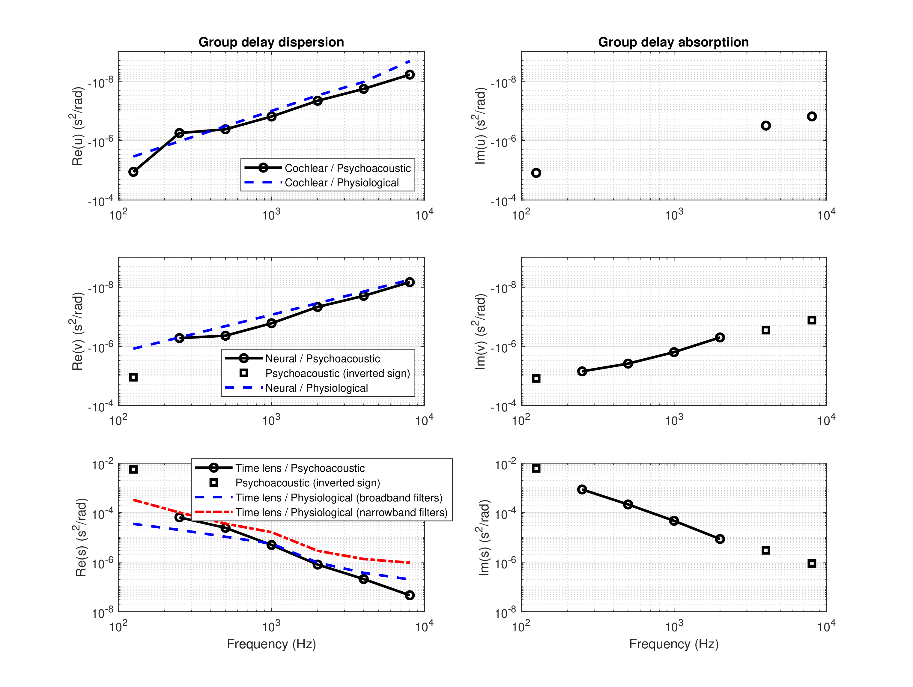
Figure F.1: The cochlear (\(u\)) and neural (\(v\)) group delay-dispersions and the time-lens curvature (\(s\)) based on the psychoacoustic model of beating threshold (Eq. §F.1), phase curvature data (Eq. §F.2), stretched octave (Eq. §F.7), and double Gabor pulse gap detection (Eq. §F.11), plotted in black circles / solid lines. The real parts are displayed on the left. At the lowest frequency (125 Hz), the values of \(v\) and \(s\) have inverted sign and are presented as black squares. For comparison, the estimates from the main text that are based on electrophysiological human and physiological animal data (§11) are displayed in blue dashed lines on the left. In addition, the two most used physiological estimates of the time lens curvature—the broad-filter (blue dash) and narrow-filter (red dash-dot) large-curvatures are displayed on the bottom left. The imaginary parts that correspond to group-delay absorption are displayed on the right (black circles / solid lines) without a physiological counterpart. Between 250 and 2000 Hz, \(u\) is real. Inverted-sign values in both \(v\) and \(s\) are marked with the disconnected black squares.
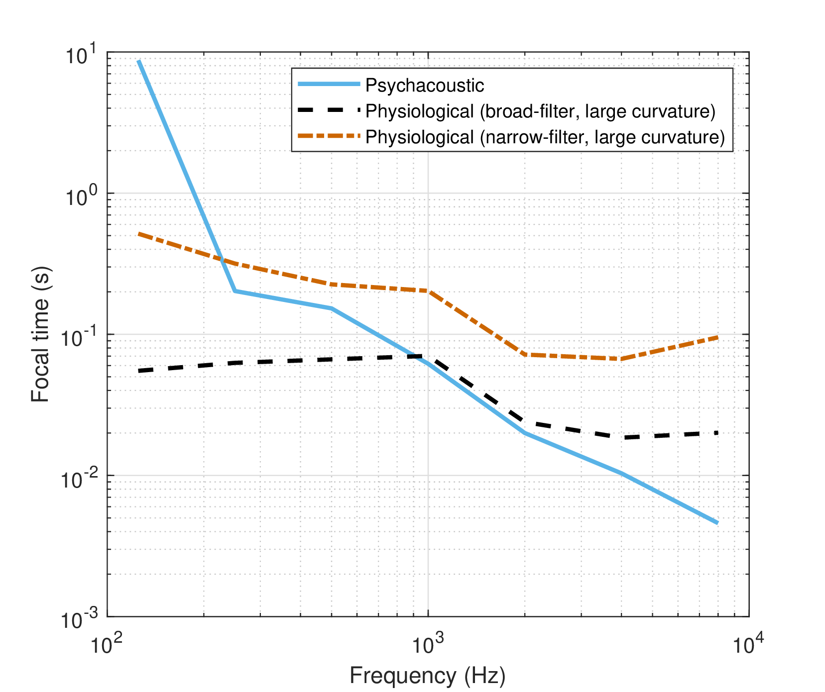
Figure F.2: The focal time \(f_T = 2\omega_c s\) corresponding to the (real part of the) time-lens curvature \(s\). The present psychoacoustic estimate is compared with the two limiting physiological estimates of the broad-filter curvature and the narrow-filter large-curvature time lenses.
F.2.2 Complex solutions?
The biggest challenge in the proposed solution is that it produces complex values in all parameters and frequencies, except for three frequencies of \(u\). The imaginary absorptive parts of the parameters are of about one order of magnitude larger than the respective real dispersive parts of all three parameters (Figure §F.1, right-hand plots). Their existence, even if troubling at first sight, is physically appropriate, given the causality/dispersion relations (Kramers-Kronig relations), which tie together the real and imaginary parts of any causal, linear, time-invariant medium (§3.4.2). While absorption was mentioned early in the original derivation in the text (§10), it was conveniently neglected (as is the convention in imaging optics) and did not seem to be necessary to obtain good fit of the parameters. Additionally, positive absorption terms of the form \(\exp(\alpha”\zeta \omega^2/2)\), where \(\alpha”\zeta > 0\) (unlike the imaginary values in Figure §F.1, including the time-lens curvature), would make the expressions intractable in closed-form if they are included in integrals (§B.2). Therefore, with the present knowledge of the system and theory, it is uncertain whether the various expressions derived for the psychoacoustic effects (mainly the phase curvature and gap detection) should hold in general for complex parameters. In principle, large group-delay absorption may further rotate the signal in the phase space, when it is combined with dispersion191.
One way to test the significance of the imaginary part on the system parameters is by comparing real-numbered predictions done with the complex valued solutions and those done with their real parts only. Two examples that were used in the text are repeated here and are displayed in Figure §F.3. On the left, the double-click gap detection predictions of Eq. §15.1 (same as Eq. §F.11 with \(T_1=0\)), led earlier to plausible temporal thresholds, at least between 1000 and 8000 Hz, where the predicted range was approximately as suggested by the rule of thumb of 2–3 ms (§15.6). Using only the real part of the new estimates of the dispersion parameters, the gap detection thresholds at all frequencies turn out shorter than with the physiological estimates, except for at 125 Hz. In contrast, using the full complex values leads to an increase and overestimation of all thresholds except for the 125 Hz value.
The temporal modulation transfer function (TMTF) cutoff frequencies are compared on the right of Figure §F.3, similarly to Figure §13.2. Both coherent and incoherent real-parameter psychoacoustic estimates are of lower frequencies than the physiological estimate. The complex-parameter incoherent estimate is implausible, since it predicts cutoff frequencies that are much higher than the coherent limits. Interestingly, the real coherent estimate at two out of three low carrier frequencies dodges the over-modulation problem that was highlighted in §12.5.2, since its predicted bandwidth is much lower than the carrier frequency by a factor of five.
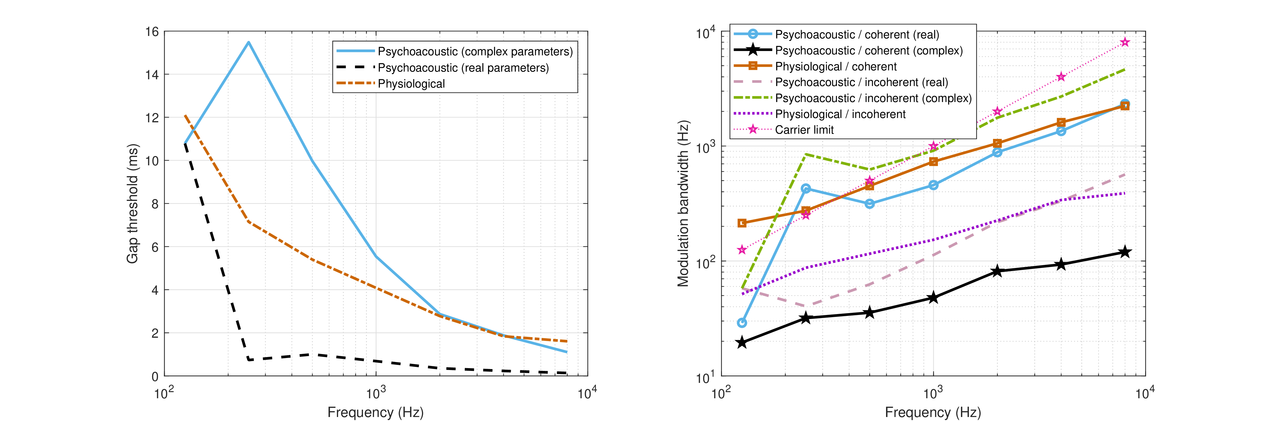
Figure F.3: Comparison of dispersive computations using real and complex parameters. Left: Double-click audibility threshold according to three estimates, using Eq. §15.1. The solid blue curve was computed using the complex parameter values shown in Figure §F.1, whereas the black dashed curve used their real parts only. The physiological model lies in the middle in dash-dot red. Right: Predicted cutoff frequencies of coherent and incoherent temporal modulation transfer functions (TMTFs). The physical bound of over-modulation on the carrier is marked with dotted purple stars.
F.2.3 Low-frequency inversion
The group-delay dispersion sign changes in \(v\) and \(s\) account for the physiological curvature anomalous behavior in the Oxenham and Dau (2001a) lowest frequency measurement. Moreover, it may constitute a parallel to the cat's auditory nerve results in Carney et al. (1999), who found that at low frequencies the impulse response glide slope changed sign from rising at high frequencies (\(>1500\) Hz) to approximately flat between 750 and 1500 Hz, and to falling at low frequencies (\(<750\) Hz). These frequency ranges of the cat can be scaled to human above 530 Hz (high), 260-530 Hz (flat), and below 260 Hz (low) (Greenwood, 1990). However, no sign inversion was identified in humans in the psychoacoustic curvature experiments by Oxenham and Dau (2001a). The difference might lie in the extra neural dispersion that was excluded by Carney et al. (1999), as they tapped the signal in the auditory nerve and not in the inferior colliculus. The sign inversion may mean that at some point in the apical region the signal is in sharp focus.
Alternatively, the sign inversion in \(v\) and \(s\) may be erroneous. The inversion may be a result of imprecise low-frequency data of one of the parameters used in the test, or caused by another inconsistency. Such numerical instability may be the case as with some choices of psychoacoustic data (e.g., different beating thresholds), if it is \(u\) that is inverted, rather than \(v\) and \(s\). However, it is unlikely that \(u\) changes sign, because this would imply that the group delay of the cochlea decreases at very low frequencies, which seems unreasonable, if energy to the inner hair cells is transmitted sequentially through the traveling wave. Sign changes in neural dispersion also seem somewhat less easy to justify. In contrast, it is perhaps possible that the time lens loses its phase-modulation capability close to the helicotrema, where the wide basilar membrane may become less compliant and is subjected to different boundary conditions than in the basal turns (note that a large value of \(s\) entails a small effect of the lens).
F.2.4 Magnification
The magnification has two alternative expressions that are exactly equal only when the system is in sharp focus, \(M = \frac{s+v}{s}\) (the actual magnification factor) and \(M_0 = -\frac{v}{u}\) (real parts assumed everywhere). Given the phase curvature as was measured by Oxenham and Dau (2001a) and others, we know that the system has to be permanently defocused, which means that \(M \neq M_0\) (§12.3). This is the case in both the psychoacoustic and the physiological estimates. There are three main differences between the two models. First, \(M\) is much closer to unity in the new estimate, similar to the two large-curvature time lens physiological estimates, which perfectly explains (by design) the stretched octave data and the musical range. Second, as a result, \(M_0\) changes sign around 160–200 Hz—with an unknown effect. It should be noted that two complex roots of Eq. §F.14 were ruled out partly because of their estimated \(M_0 \approx 0\), which could not be justified. Finally, the new \(M_0\) is much closer to -1 and is fairly constant, given that \(u\) and \(v\) are of very similar magnitudes. \(M_0\) was used in §13.2.1 to approximate time-invariant impulse response.
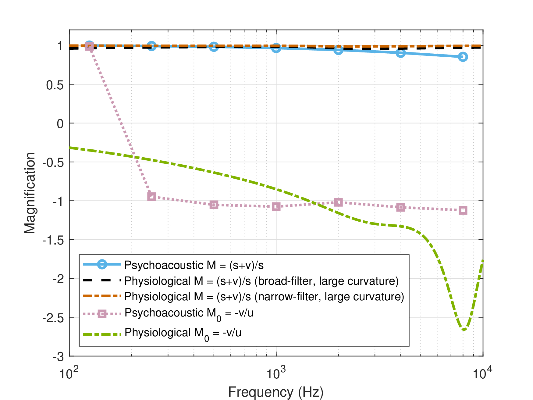
Figure F.4: Different estimates for the two magnification definitions of the imaging system, \(M = \frac{s+v}{s}\) and \(M_0 = -\frac{v}{u}\). When the system is in sharp focus \(M=M_0\). In both psychoacoustic and physiological estimates \(M \approx 1 \), especially in the large-curvature estimate. According to the psychoacoustic estimate \(M_0 \approx -1\), but since \(v\) changes sign at low frequencies, then \(M_0\) changes sign at around 160–200 Hz as well.
F.3 General discussion
The psychoacoustic solution proposed here is almost completely independent of the previous solution that was based on physiological data, except for the phase curvature measurements that were used in both methods. At the level of rigor obtained here, it provides only a partial validation to the temporal imaging theory in its current formulation. First, the only plausible solutions are complex, which may or may not relate to physical absorptive attributes of the auditory medium. At this stage, there is no method to map it to any known measurements. Then, using the real part only is not always justified, as some derivative figures (e.g., double-click detection thresholds) are highly sensitive to the imaginary part as well—probably because of its significant order of magnitude relative to dispersion. That said, most real-valued results are relatively consistent with the physiological data. The one exception is at the lowest frequency band, which shows a sign change in one or more parameters. This might be consistent with the anomalous response observed in the Oxenham and Dau (2001a) measurements and in cat data from Carney et al. (1999), although we would expect to see sign inversion taking place at a higher frequency—something which was not seen in the data. It suggests that the low-frequency range may be governed by somewhat different equations than were used in this work.
Another interesting result from this work relates specifically to the time-lens curvature. Its physiological estimation process (§11.6) required some speculative assumptions that nevertheless relied on five studies with what appeared to be unmistakable phase modulation in the organ of Corti. Assuming scaling between animal data and humans, we obtained wide bounds of the curvature, but picked mainly those that correspond to either broad or narrow auditory filter response in humans. Predictions that were based on these values were sometimes closer using one curvature (small or large) than with the other, but were generally similar. The psychoacoustic curvature estimate is somewhere in between the two, as it is closer to the narrow-filter physiological estimate at low frequencies and to the broad-filter curvature above 1000 Hz. Incidentally, the psychoacoustic estimate is far from the small-curvature estimate that was ruled out in much of the analyses throughout this work, for producing all sorts of outliers and unlikely sign inversions. However, as noted earlier, it is more likely than not that the time-lens curvature is adaptive by virtue of the medial olivocochlear reflex accommodation. In this case, small-curvature values may better fit conditions that have not been explored here.
Should the above model and equations prove correct over time, they suggest an indirect way to estimate the dispersion parameters noninvasively. The estimates may even reveal individual differences, analogous to refractive errors in vision. Beating, Gabor pulse detection, and stretched octave tests are relatively easy to administer, even if not particularly easy to obtain stable results from. But the phase curvature testing procedure, as administered by Oxenham and Dau (2001a), is very tedious and will have to be made shorter and simpler in order to be suitable for human data collection on a larger test sample. An alternative technique has been recently proposed by Rahmat and O'Beirne (2015) and cuts the average test time by a factor of 5.5. Importantly, administering such a comprehensive test battery should be done at a uniform sound pressure level—a control that was not available to us here and has undoubtedly detracted from the overall accuracy of the results.
\let
Footnotes
191. Note that first-order absorption coefficient that is linearly dependent on frequency has an effect on phase similar to dispersion, but is not considered in this work.
References
Carney, Laurel H, McDuffy, Megean J, and Shekhter, Ilya. Frequency glides in the impulse responses of auditory-nerve fibers. The Journal of the Acoustical Society of America, 105 (4): 2384–2391, 1999.
Gabor, Dennis. Theory of communication. Part 1: The analysis of information. Journal of the Institution of Electrical Engineers-Part III: Radio and Communication Engineering, 93 (26): 429–457, 1946.
Greenwood, Donald D. A cochlear frequency-position function for several species"29 years later. The Journal of the Acoustical Society of America, 87 (6): 2592–2605, 1990.
Jaatinen, Jussi, Pätynen, Jukka, and Alho, Kimmo. Octave stretching phenomenon with complex tones of orchestral instruments. The Journal of the Acoustical Society of America, 146 (5): 3203–3214, 2019.
Oxenham, Andrew J and Dau, Torsten. Towards a measure of auditory-filter phase response. The Journal of the Acoustical Society of America, 110 (6): 3169–3178, 2001a.
Plomp, Reinier. The ear as a frequency analyzer. The Journal of the Acoustical Society of America, 36 (9): 1628–1636, 1964a.
Plomp, R and Steeneken, HJM. Interference between two simple tones. The Journal of the Acoustical Society of America, 43 (4): 883–884, 1968.
Rahmat, Sarah and O'Beirne, Greg A. The development of a fast method for recording Schroeder-phase masking functions. Hearing Research, 330: 125–133, 2015.