 )
)Appendix A
Examples of realistic coherence functions of acoustic sources
A.1 Introduction
This appendix supplements some of the statements made throughout the review of coherence theory that are relevant for acoustics and hearing (§8)—primarily in the sections about realistic acoustic sources (§8.3.2) and room acoustics (§8.4.2). The overarching goal of the examples in this appendix is to demonstrate that partial coherence is prevalent in relatively ordinary conditions—a claim that is repeatedly made throughout this work. As information supporting this claim could not be conveniently gathered from available literature, it was deemed instructive to generate the required data using available recordings. The interpretation of some of the effects is not always straightforward, especially since several critical factors go into every analysis—frequency-dependent coherence, nonstationarity of the sources, reverberation time, integration time of the coherence function, the analysis filter, and more. The challenge in interpretation is exacerbated because the relative weighting and exact interplay between these factors are unknown with respect to hearing. Nevertheless, it is the hope here that the figures below will serve the immediate purpose of showing how real-world acoustic fields are not black or white—they are neither coherent nor incoherent, but are generally a mixture of both: they are partially coherent.
The basic relation used throughout this work to obtain the coherence function is the correlation function:
| \[ \Gamma(\boldsymbol{\mathbf{r_1}},\boldsymbol{\mathbf{r_2}},\tau) = \frac{1}{2T} \int_{-T}^T p^*(\boldsymbol{\mathbf{r_1}},t)p(\boldsymbol{\mathbf{r_2}},t+\tau)dt \] | (A.1) |
which is integrated over a finite duration \(2T\) that in the limit of \(T \rightarrow \infty\) converges to the ensemble average value, if stationarity is satisfied. When \(\boldsymbol{\mathbf{r_1}}=\boldsymbol{\mathbf{r_2}}=\boldsymbol{\mathbf{r}}\), \(\Gamma(\boldsymbol{\mathbf{r,r}},\tau)\) is referred to as the self-coherence function, and then Eq. §A.1 assumes the form of a standard autocorrelation function. Eq. §A.1 is normalized by the root mean square of both signals according to:
| \[ \gamma(\boldsymbol{\mathbf{r_1}},\boldsymbol{\mathbf{r_2}},\tau) = \frac{\Gamma(\boldsymbol{\mathbf{r_1}},\boldsymbol{\mathbf{r_2}},\tau)}{\sqrt{\Gamma(\boldsymbol{\mathbf{r_1}},\boldsymbol{\mathbf{r_1}},0)}\sqrt{\Gamma(\boldsymbol{\mathbf{r_2}},\boldsymbol{\mathbf{r_2}},0)}} \] | (A.2) |
to obtain the complex degree of coherence, \(\gamma(\boldsymbol{\mathbf{r_1}},\boldsymbol{\mathbf{r_2}},\tau)\).
In most of the following analyses, we are interested in the transition between coherence (\(\gamma = 1\)) and incoherence (\(\gamma = 0\)). In the room acoustic and psychoacoustic literature, it was indirectly assessed using the effective duration, which is defined as the duration for a 10 dB drop from the peak of the autocorrelation function, which is always coherent at \(\tau = 0\) and drops for larger lags. This measure has been shown to correlate with various subjective measures, but the choice of 10 dB does not seem to have been justified in literature and appears to be somewhat arbitrary. In contrast, the coherence time as is defined in coherence theory (§8.2.4) is computed at the half power point (-3 dB). This duration also corresponds to the point at which the coherent and incoherent components in the total (partial) coherence function are exactly equal, according to Eq. §8.22: \(I_{coh/}I_{incoh} = |\gamma(\boldsymbol{\mathbf{r_1}},\boldsymbol{\mathbf{r_1}},\tau)/|(1-|\gamma(\boldsymbol{\mathbf{r_1}},\boldsymbol{\mathbf{r_1}},\tau)|)\). Therefore, we shall make a distinction between the coherence time (-3 dB) and the effective duration (-10 dB). As a working hypothesis, we will assume that complete (subjective) coherence is obtained for delays shorter than the coherence time \(\tau<\Delta \tau\) and subjective complete incoherence is obtained for delays longer than the effective duration \(\tau > \tau_e\). The broad margin in between corresponds to subjective partially coherent sound. The exact cutoff in auditory relevant measures is, of course, unknown at present.
A notable and known pattern that repeats in the following measurements is that the coherence time decreases with frequency. This is a corollary of the 1/f-like distribution of the power spectrum of different sources of physical noise, which also characterizes speech and music loudness and pitch fluctuations (Van Der Ziel, 1950; Voss and Clarke, 1975).
Several sound examples from the recordings that are analyzed throughout are found in the audio demo directory /Appendix A - Coherence/.
A.2 White noise and the cohering effect of two filter types
Although the autocorrelation function is routinely applied in acoustics to broadband sources, the physical coherence function that carries information about interference between sources is well defined only for narrowband signals. In order to obtain a narrowband approximation that is required to get meaningful results out of the temporal-spatial coherence functions, it is necessary to bandpass-filter the various broadband acoustic signals. However, the choice of filter can significantly influence the output coherence function and is therefore not completely arbitrary (§8.2.8). To illustrate this effect, we shall compare the white-noise coherence function for different Butterworth and gammachirp filters. The Butterworth filters are designed to maximize the flatness of the passband magnitude, but are characterized by relatively slow rise time and frequency-dependent group delay in the flanks (Blinchikoff and Zverev, 2001; 109–117). The gammachirp filters are the standard model for the auditory filters (Patterson et al., 1987; Irino and Patterson, 1997). They are faster than the Butterworth filters and account for the asymmetry of the passband. However, they are modeled using stationary signals (pure tone and broadband maskers) and probably have an incorrect phase response (Lentz and Leek, 2001) that may not square well with some transient nonlinear characteristics. The passband in both cases is set according to the equivalent rectangular bandwidth of the auditory filters (Glasberg and Moore, 1990):
| \[ ERB = 0.108f + 24.7 \,\,\, \mathop{\mathrm{Hz}} \] | (A.3) |
for frequency \(f\) in Hz.
White noise, in theory, has a zero coherence time in the limit of infinite bandwidth of the noise. However, as was proven in §8.2.8 and was originally shown in Jacobsen and Nielsen (1987), the choice of filter bandwidth affects the measurement, and hence, the apparent coherence of the source. This is illustrated in Figure §A.1. The pre-filtered autocorrelation of a 5 s pseudo-random white noise is shown in all plots as the blue trace. The negative half plane of the autocorrelation is omitted due to its symmetry. The autocorrelation of Eq. §8.84 was calculated with \(T=0.1\) s and 50% overlap between analysis frames and then averaged over all frames. The envelope of the obtained autocorrelation that appears in each plot was extracted using the magnitude of the Hilbert transform of the average autocorrelation function on all frames (Ando et al., 1989; D'Orazio et al., 2011). The coherence time \(\Delta \tau\) (seen on the plot top right corners) was calculated by finding the duration it took the envelope to drop by 3 dB from its peak value. The effective duration was found by fitting a linear curve to the logarithmic envelope of the coherence function between 0 and -5 dB and extrapolating it to -10 dB, in accord with the standard definition of effective duration (Ando, 1985).
In all plots, the coherence time \(\Delta \tau\) and effective duration \(\tau_e\) are smaller than 0.15 ms179. Butterworth filtering (2nd-, 4th-, 6th-, and 8th-order) is displayed in plots A, C, and E for center frequencies of 100, 500, and 2500 Hz, respectively. In all cases, the coherence time (and effective duration) increases as the center frequency decreases. Both \(\Delta \tau\) and \(\tau_e\) are approximately doubled when the filter order is increased from 2nd- to 6th-order. The effect of an 8th-order filter appears more unpredictable, though. The gammachirp filtering (plots B, D, F) is more predictable and has much shorter times associated with it. However, the filter orders are not directly equivalent and (the standard) 4th-order gammachirp results in approximately the same coherence time and effective duration values as the 2nd-order Butterworth, in all cases.
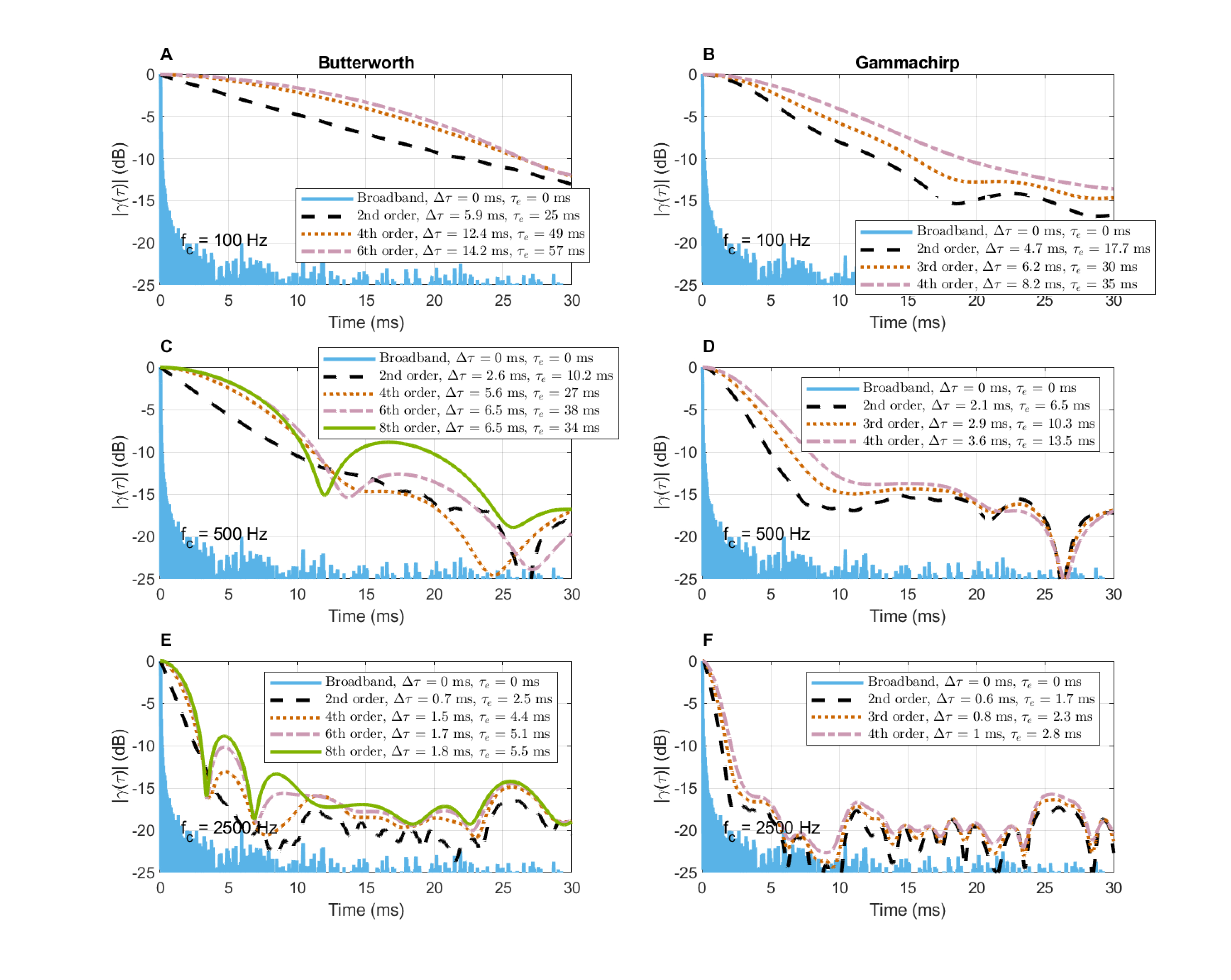
Figure A.1: Demonstration of the cohering effect of two different types of filters with bandwidths set according to the ERB in Eq.§A.3, in four orders each. On the right are band-pass Butterworth filters of 2nd, 4th, 6th, and 8th order (standard bandpass orders are always even). On the left are Gammachirp filters of 2nd, 3rd, and 4th orders. White Gaussian noise of 5 s was used as signal and the integration time was 100 ms, in all cases.
Regardless of the specific type and order of filter selected, the effect on coherence is unmistakable, as even white noise that enters as a completely incoherent signal, leaves the filter as partially coherent. This is an important result that will be used at several points in the main text.
The 6th-order Butterworth filter will be used throughout this appendix, as it has a known phase response and has sufficient frequency resolution to reflect features visible in the broadband spectrum. Its downside appears to be that at short coherence times and frequencies, the filter dominates the coherence function response and makes it excessively long—it likely exaggerates the low-frequency signal coherence time. Therefore, the values below should be interpreted in a comparative and relative sense rather in the strict absolute manner.
A.3 Effect of integration time
Examples of the effects of the integration time of the correlation integral (Eq. §A.1) are shown in Figure §A.2 for an acoustic source that is presented in §A.6.1—a saxophone that tends to produce long notes of high coherence. The effect of varying the integration constant duration \(T\) between 25 and 400 ms is frequency dependent in the saxophone example, since longer \(T\) results in longer coherence time at low frequencies (plot A), while it is maximized with \(T=100\) ms at the midrange frequency (plot B), and is unaffected at the highest frequencies (plot C). The effective duration is somewhat different, as it is more sensitive to fluctuations. The shortest integration times (25 and 50 ms) are clearly too short to capture significant portions of the signal that can reveal relevant coherent patterns. The longest integration times (200 and 400 ms) do not necessarily add critical information to the analysis that is maybe more suitable for sustained and stationary sounds.
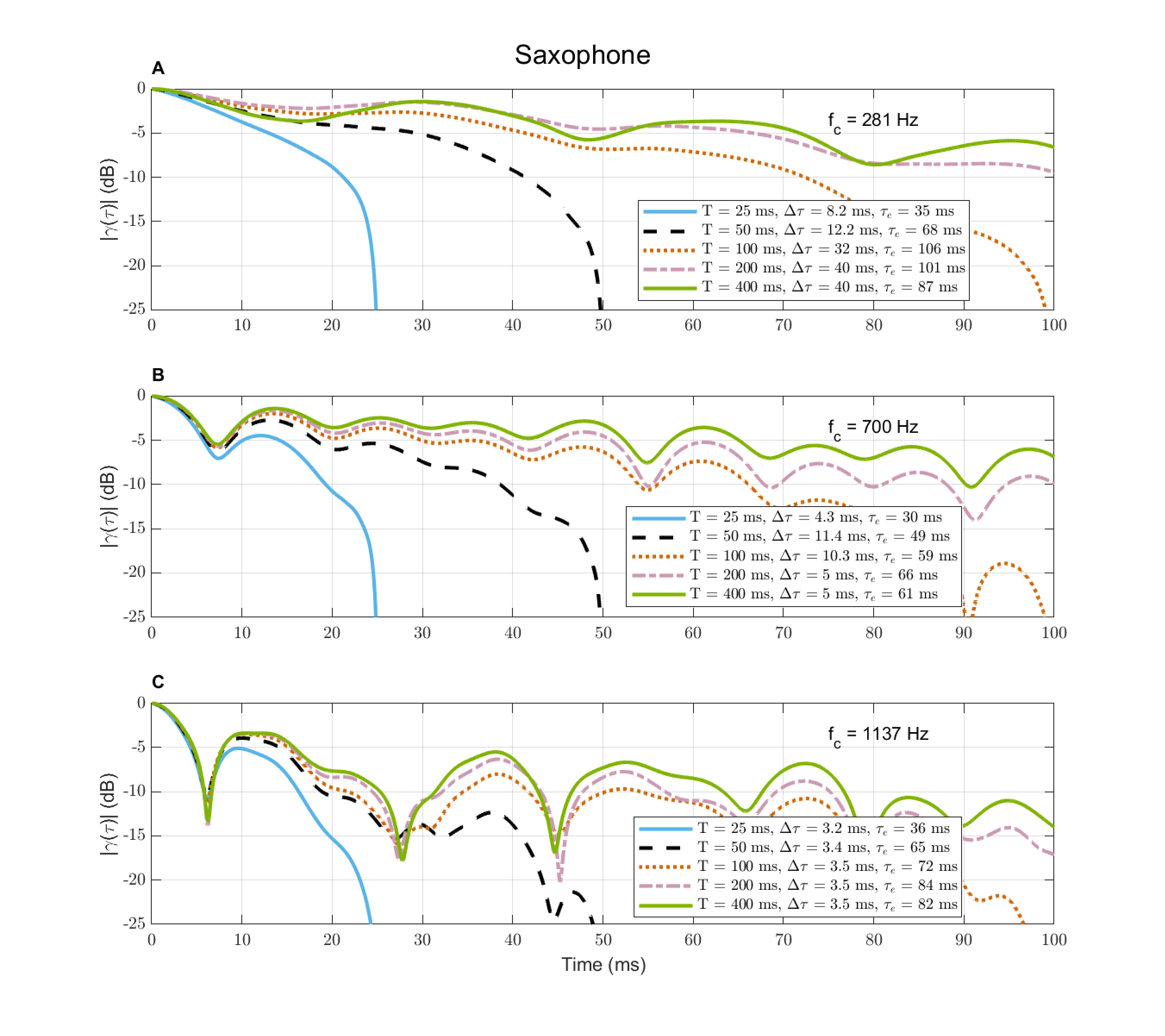
Figure A.2: The effect of the integration time \(T\) on the same autocorrelation function as is in plots A, B, and C, for a 6th-order Butterworth filter, which has been used as a standard in this appendix. The coherence time \(\Delta\tau\) and effective duration \(\tau_e\) are displayed for all conditions.
A.4 Stationarity and nonstationarity
It was mentioned several times in the text that the assumption of stationarity does not hold for typical acoustic signals that function as auditory stimuli. Nonstationarity complicates the analysis and sets many of the results obtained using the stationarity assumption as limiting cases. In the figure below (§A.3), the nonstationarity of the seven sound samples that have been used in this appendix and are presented in the subsequent sections, is analyzed using a simple measure. Kapilow et al. (1999) proposed three stationarity indices to facilitate various algorithms of speech processing, which can produce severe artifacts if used to process sound segments that are nonstationary (mainly phonemic boundaries). The simplest index proposed in the paper (\(C_n^1\) in Kapilow et al., 1999) is based on the root mean square (RMS) level difference between consecutive analysis windows of the sound:
| \[ NS = \frac{|p_n - p_{n-1}|}{p_n + p_{n-1}} \] | (A.4) |
where \(p_n\) refers to the RMS level of the pressure in time frame \(n\), which was set here to be 100 ms long. When the difference term in the numerator is 0, the signal does not vary in level, which entails stationarity. If it maximally varies, \(NS\) is 1. Therefore, it seems appropriate to think of this measure as a nonstationarity index rather than a stationarity index.
In Figure §A.3, the plots on the left refer to the four sources used in §A.5 and the plots on the right to the other three sources that are used in §A.6.1. The vibraphone note (plot A)—being tonal and sustained—appears stationary as \(NS \approx 0\). In plots B, D, and F, the nonstationarity of pseudorandom white noise is displayed in black and shows zero nonstationarity, as expected. All other examples are nonstationary to different degrees, but musical sounds (vibraphone, saxophone, singing) appear to be more stationary than others. Speech and laughter have particularly erratic nonstationarity patterns. In the case of the sources on the right of Figure §A.3, alternative microphone positions were all plotted for comparison and exhibit reasonably close figures, which implies that moderate reverberation does not have a strong effect on the inherent stationarity of the signal. In fact, in some cases the remote positions appear more nonstationary on average than the near position (tom drum), whereas it is the opposite in other cases (singing).
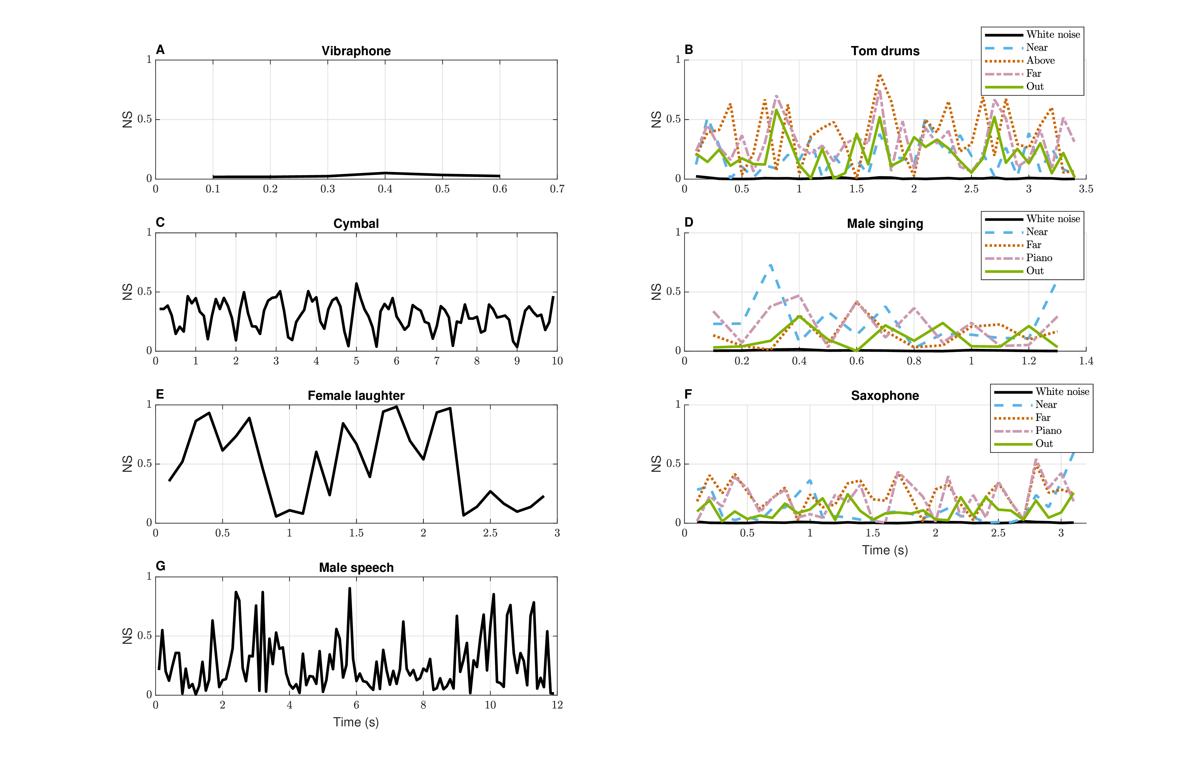
Figure A.3: The nonstationarity index of the seven sources used throughout the appendix, according to Eq. §A.4. The sources were analyzed in 100 ms consecutive frames. On the right hand side, each source is analyzed in all four microphone positions available, which generally showed similar patterns. For comparison, the black curves on the right-hand figures (B, D, and F) shows the nonstationarity index of pseudo-random white noise of identical duration, which approaches zero with \(NS \approx 0.005\).
The nonstationarity estimated in the various cases suggests that using stationary coherence function of the form of Eq. §A.1 is not strictly correct. This equation assumes that the correlation operation is time invariant, so that the signals can be compared (correlated) at any two points \(t_1\) and \(t_2\) and produce the same results. This gives rise to the time-invariant time delay variable \(\tau\). However, the nonstationarity entails time dependence, so relevant signals have to be evaluated with the two time coordinates instead. For simplicity, we do not pursue this approach here, but show only some examples of the time-dependent effective duration in the next section.
A.5 Four narrowband coherence-time examples
From §8.3.2, it appears that a relatively fragmentary sample of effective durations of various acoustic sources is provided in literature, and almost none of acoustic coherence times. Critically, the available reports have exclusively focused on the autocorrelation of the full (broadband) spectrum, which is useful in the discussion of pitch and broadband periodicity, but produces difficulties in interpreting nonstationary broadband sounds. Broadband autocorrelation peaks may correspond to different sounds associated with specific sources (e.g., certain musical instruments in an ensemble), or within sources when their spectra are complex and comprise multiple modes. As the auditory system decomposes the broadband signal to narrowband channels, there may be some information that cannot be garnered from such broadband analyses. Therefore, in order to anchor the subsequent discussions with relevant data, narrowband autocorrelation analysis is provided for four acoustic sources.
The narrowband autocorrelation curves in the next four Figures (§A.4, §A.5, §A.6, and §A.7) were all computed using identical methods as in §A.2, and are displayed in a uniform format. The center frequencies were selected by analyzing the spectrum (plots I). This was done in order to have examples that contrast different coherence time characteristics in different bands. The median value of the effective duration \(\tau_e\) values are printed in plots B, D, F, where changes are shown along the duration of the recording. The corresponding narrowband filtering was achieved with 6th-order bandpass Butterworth filters, set with the equivalent rectangular bandwidth of auditory filters with the center frequency (Eq. §A.3).
Both \(\Delta \tau\) and \(\tau_e\) are dependent on the choice of the integration time \(T\). The particular choice of \(T=0.1\) s produced values that subjectively reflected the author's impression of coherence from listening to the sounds. However, different choices of \(T\) would retain the relative differences between the different coherence functions, as was seen in §A.3. The spectrum of the sound was obtained using the same time frames, using fast-Fourier transform (FFT) with 4096 points (plots I). Finally, the broadband autocorrelation is displayed in plots J along with its associated effective duration. Corresponding audio demos to the samples that are presented in this analysis are found in the demo directory /Appendix A - Coherence/Narrowband coherence/.
Figure §A.4 shows the analysis of a sustained complex tone (B4 = 494 Hz, 0.7 s) of a vibraphone180 in four frequency bands. The fundamental and the second octave overtone (1986 Hz) were selected as the most coherent modes (plots A–B and E–F, according to the spectrum in plot J), whereas two other frequencies (1100 and 5800 Hz) that are not associated with apparent overtones are plotted in C–D and G–H. The coherence times are an order of magnitude longer in overtones (\(\sim\)45 ms) than in non-overtone frequencies (\(\sim\)1–3 ms). The audio version of the fundamental sounds almost indistinguishable from a pure tone, whereas the overtone has a subtle timbral variation in its attack, despite a very small (4 ms) decrease in mean \(\Delta \tau\) (but not in the running \(\tau_e\)) compared to the fundamental. For the 1100 Hz (plots C and D), the mean \(\Delta \tau\) is much shorter (3.5 ms) despite a long \(\tau_e\) (147 ms), which reveals a step in the corresponding effective duration curve (plot B). It is also audible in the faint recording, which starts with a clunky noise-like attack sound before it becomes more tonal. The last frequency (plots G and H) has much shorter \(\Delta\tau\) and \(\tau_e\) (\(<2.5\) ms), which indeed sounds like noisy-clicky sound with no discernible pitch.
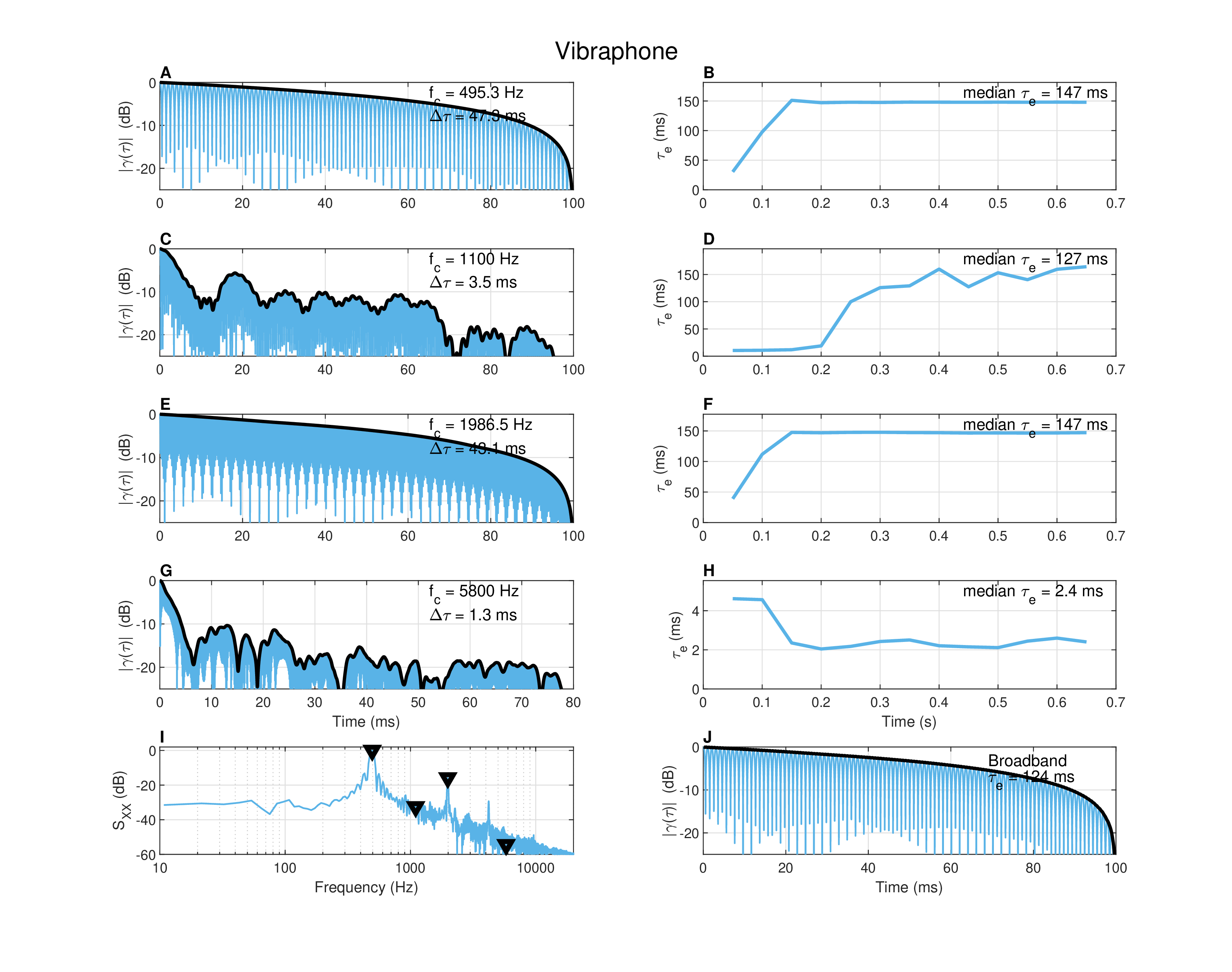
Figure A.4: Autocorrelation of a vibraphone note (B4 = 494 Hz) of duration 0.7 s, recorded in near-field in a dry room. The integration time is \(T = 0.1\) s. The average autocorrelation curves are plotted on a dB scale. The coherence time (\(\Delta \tau\)) is the -3 dB point on the Hilbert envelope of the coherence function. The effective duration (\(\tau_e\)) is extrapolated to the -10 dB on the envelope (see text). Bandpass filtering was used to obtain narrowband autocorrelation curves with center frequency as marked in plots A, C, E, and G and bandwidth equal to the equivalent rectangular bandwidth of a corresponding auditory filter. The corresponding plots B, D, F, and H give the running effective duration and its median value for that frequency band. The frequencies were selected from the spectrum (plot I), where they are marked with triangles. The broadband autocorrelation function appears in plot J.
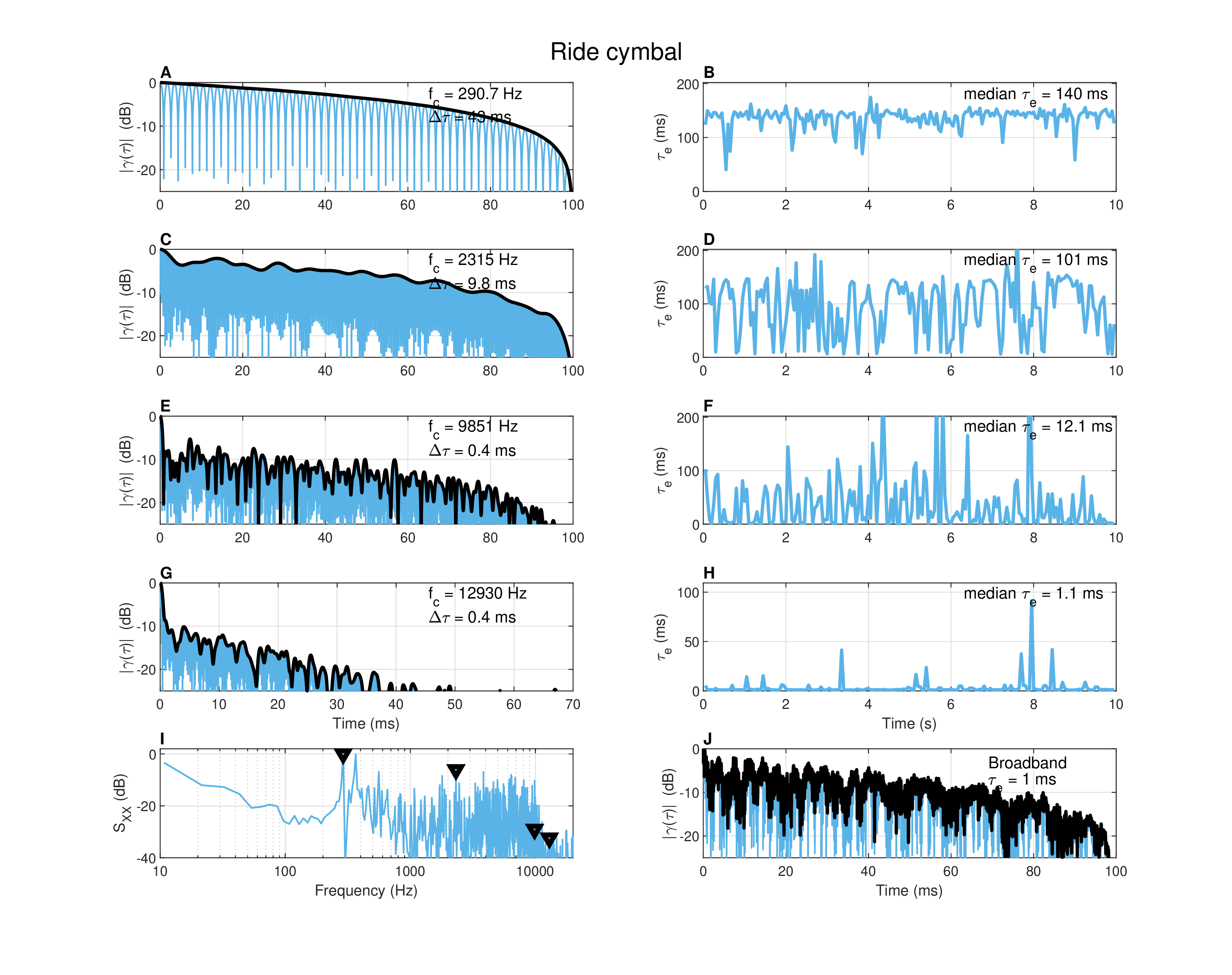
Figure A.5: Autocorrelation of a ride cymbal being played with a drum stick for 10 s, recorded with a close microphone in a dry studio. The measurement details are given in Figure §A.4 and in the text.
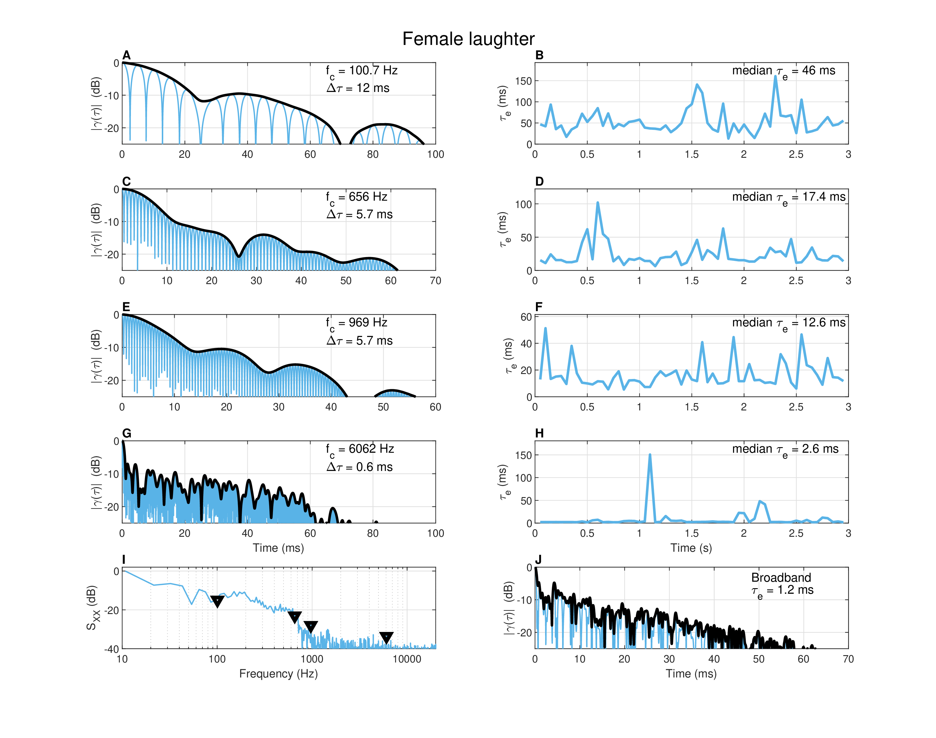
Figure A.6: Autocorrelation of female laughter of 3 s duration, recorded in a standardized audiometric booth. See measurement details in Figure §A.4 and in the text.
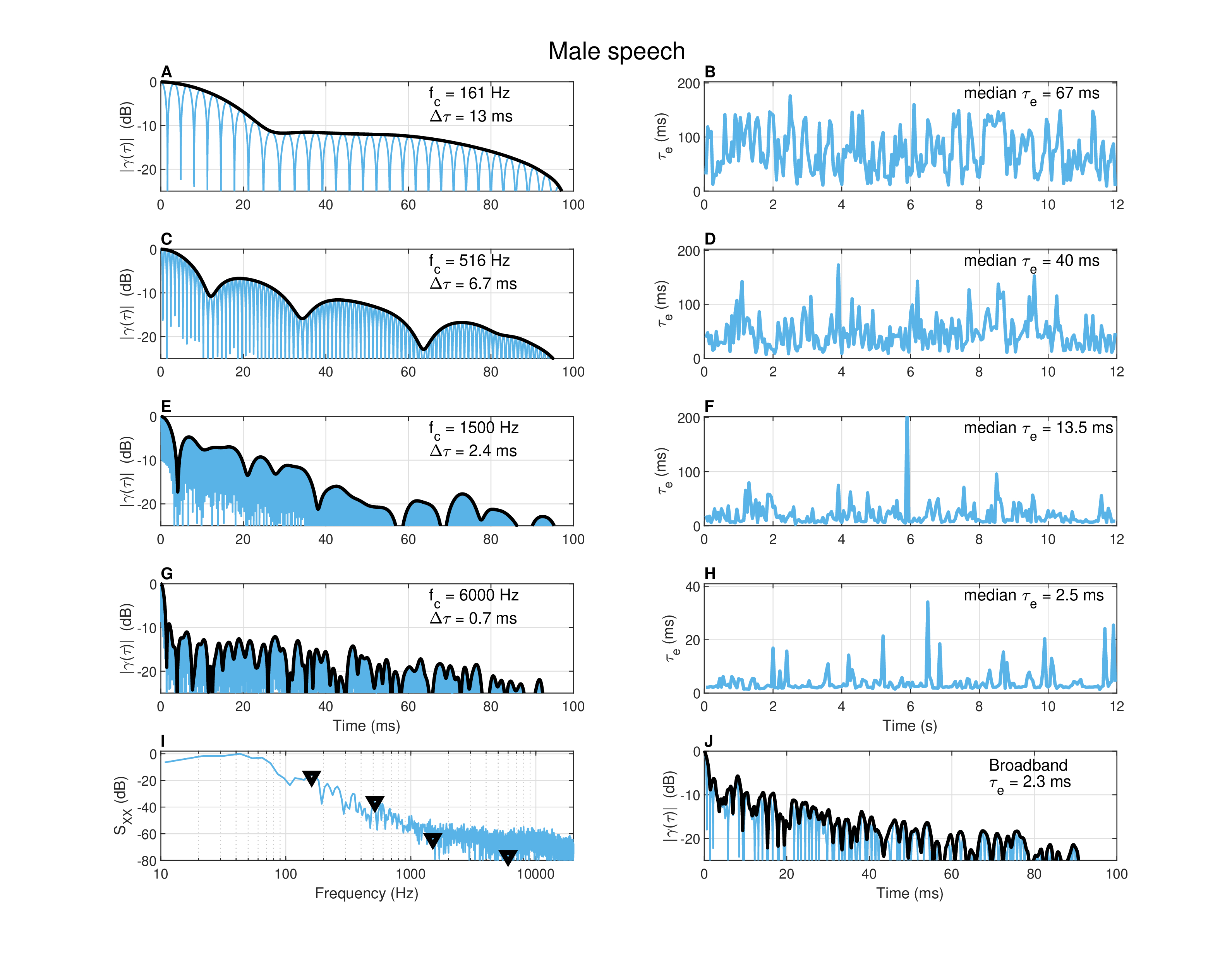
Figure A.7: Autocorrelation of male speech of 12 s duration, recorded in a standardized audiometric booth. See measurement details in Figure §A.4 and in the text.
The second sound analyzed in Figure §A.5 is musical but not tonal—a large (22”) ride cymbal mounted on a stand that was struck with a drumstick in an unsteady rhythm. It was recorded in near-field and dry studio conditions. Cymbals are characterized by high modal density and distinct high-frequency attack sound that are excited by the drumstick. The lowest eigenfrequency (290 Hz, plots A and B) gave coherence time that is comparable to the vibraphone modes (43 ms), which nevertheless sounds like a hollow tone—somewhat less clear and steady than a pure tone—which never decays significantly between hits. The next frequency band (2315 Hz, plots C and D) sounds dirtier and retains an audible indication for the drumstick hits with variable impact levels, although it is still largely sustained, with shorter coherence time (9.8 ms). The last two frequencies are of very short coherence time (0.4 ms) and are neither tonal nor sustained, as the impulsive hits are distinctly heard. The highest frequency (13 kHz, plots G and H) sounds like faint dirty clicks. In this case, the decrease in coherence time with frequency is also reflective of the decrease in the decay time of high frequency modes in cymbals (Fletcher and Rossing, 1998; 652–655).
The third sound (Figure §A.6) is a 3 s female-laughter recording done in an audiometric booth in near-field conditions. Its spectrum (plot I) does not reveal clear peaks and indeed none of the narrowband recordings resembles laughter, suggesting that laughter may be described more faithfully as a modulated broadband sound than using specific normal modes, or that the modal excitation is too nonstationary to be modeled in the way presented here (cf. Bachorowski et al., 2001). Relative agreement in the decrease rate of both coherence time and effective duration was obtained in all frequencies, where the coherence time dropped from about 12 ms at 100 Hz to 0.6 ms at 6 kHz. In general, it is evident that low frequencies have longer coherence times than high frequencies, although it depends also on the particular signal contents, which seem to be highly variable, judging from the running effective duration plots.
The fourth and last sound (Figure §A.7) is a 12 s male-speech recording done in the same conditions as the female laughter from Figure §A.6. The spectrum (plot I) is rich with resonances, but only few that are prominent. Therefore, an attempt was made to pick frequencies that display the largest variance in coherence time. At 161 Hz (plots A and B), the coherence time is 13 ms and, as can be heard in the recording, it is clearly amplitude- and frequency-modulated—the latter as a result of prosodic changes of the fundamental frequency. At 516 Hz (plots C and D), the filtered recording sounds more speech-like with amplitude-modulated noisy carrier that is hardly tonal. Here the mean coherence time (6.7 ms) is much shorter than the effective duration median (40 ms). Shorter coherence time may correspond to the atonal timbre of this sound. This impression is stronger at 1500 Hz (plots E and F), where no clear peaks are observed in the spectrum, the mean coherence time is very low (2.4 ms), and the recording sounds like a deeply amplitude-modulated narrowband buzz. This is exacerbated in the last band (6000 Hz, plots G and H), where the modulated buzz is less deep and more sustained, but sounds more like a guiro than speech.
In all cases, the broadband autocorrelation (plots J in the figures) gives only partial information about the source, which masks any distinction between coherent and incoherent parts it may have. This is perhaps not surprising, because the autocorrelation in coherence theory is strictly a narrowband measure. So, in both speech recordings, the broadband coherence time estimate is conservative, in that it estimates the speech to be less coherent than it may actually be. This can be true especially for voiced phones. In contrast, the musical vibraphone note is estimated to be more coherent than not—effectively neglecting any noise-like incoherent components of the timbre.
Another recurrent observation about the data is that the running and median autocorrelation functions occasionally yield different coherence time estimates, which should be \(\Delta \tau \approx 3\tau_e/10\) for a `well-behaved' exponentially decaying self-coherence curve. While the nonstationary coherence function fine structure is captured by the running autocorrelation, it is often too erratic to be truly useful, whereas the mean and median values appear to correspond to higher-level perception of the overall sound. Either way, these differences underline the nonstationarity of even the simplest acoustic narrowband sources.
A.6 The effects of room acoustics on coherence
It is instructive to examine a few concrete examples of sounds whose coherence properties are affected by reverberation. As was stressed throughout the main text, the degree of coherence of the acoustic source can be affected by a number of factors. The primary concern in the examples below is to explore how the relative degree of coherence varies between different sources, frequency bands, and recording positions. Three sets of recordings are tested throughout: a floor tom drum181, a tenor saxophone, and a male voice singing a three-word melody. Each set was recorded in four positions within the same large studio, with different high-quality microphones. The computational methods of the various functions are identical to those presented in §A.5, but this time we present the mean coherence time and effective duration as a function of frequency.
Unlike the samples in the previous section, the signal-to-noise ratio of the following samples was not always high. Thus, apparent incoherence may be the result of sounds that are truly unrelated to the source—either noise or altogether different sources.
A.6.1 Effect of position and frequency
All the sound samples used below were recorded in a large studio (\(V\approx 800 \,\, \mathop{\mathrm{m}}^3\)) with medium reverberation time \(T_{60} \approx 1\) s. The walls and ceiling were treated with heavy absorption and each instrument was recorded using various microphone positions. One was always close (the “near” position), one was positioned somewhere in the room to capture more of the reverberant field (“far”), and another was positioned in a much smaller room that was connected through an open doorway, but far away from the source (“out”). For the tom drum, there was another position that was not as close as the “near” position and picked up the radiation from above the drum (the '`above” position). For the singing and saxophone, another microphone was placed right over an open grand-piano soundboard, close to the strings, which may have resonated with the ambient radiated sound.
Audio demos that correspond to the samples in the analysis are found in “/Appendix A - Coherence/Room acoustics/.”
Figure §A.8 shows the autocorrelation of the floor toms that were played for 3.5 s. The hi-hat cymbal was being played throughout as well, as can be heard in the above position. However, it was less dominant in all other recordings and nearly inaudible in the near position. For clarity, only the autocorrelation envelope is shown in plots A, C, and E. As can be seen in the spectrum (plot F) of the near position, it has strong normal modes below 170 Hz, but not much energy and no special features are recognized above that. The coherence time of the near recording is distinctly longer below 170 Hz, but at higher frequencies all positions seem to approximately converge to similar coherence time. This can also be seen in the frequency-dependent coherence time and effective duration plots (B and D), which appear to be nearly merged above 1000 Hz. This suggests that the degree of coherence is almost the same at these frequencies in all room positions, which can be a result of the spectral content of the source combined with its incoherent nature.
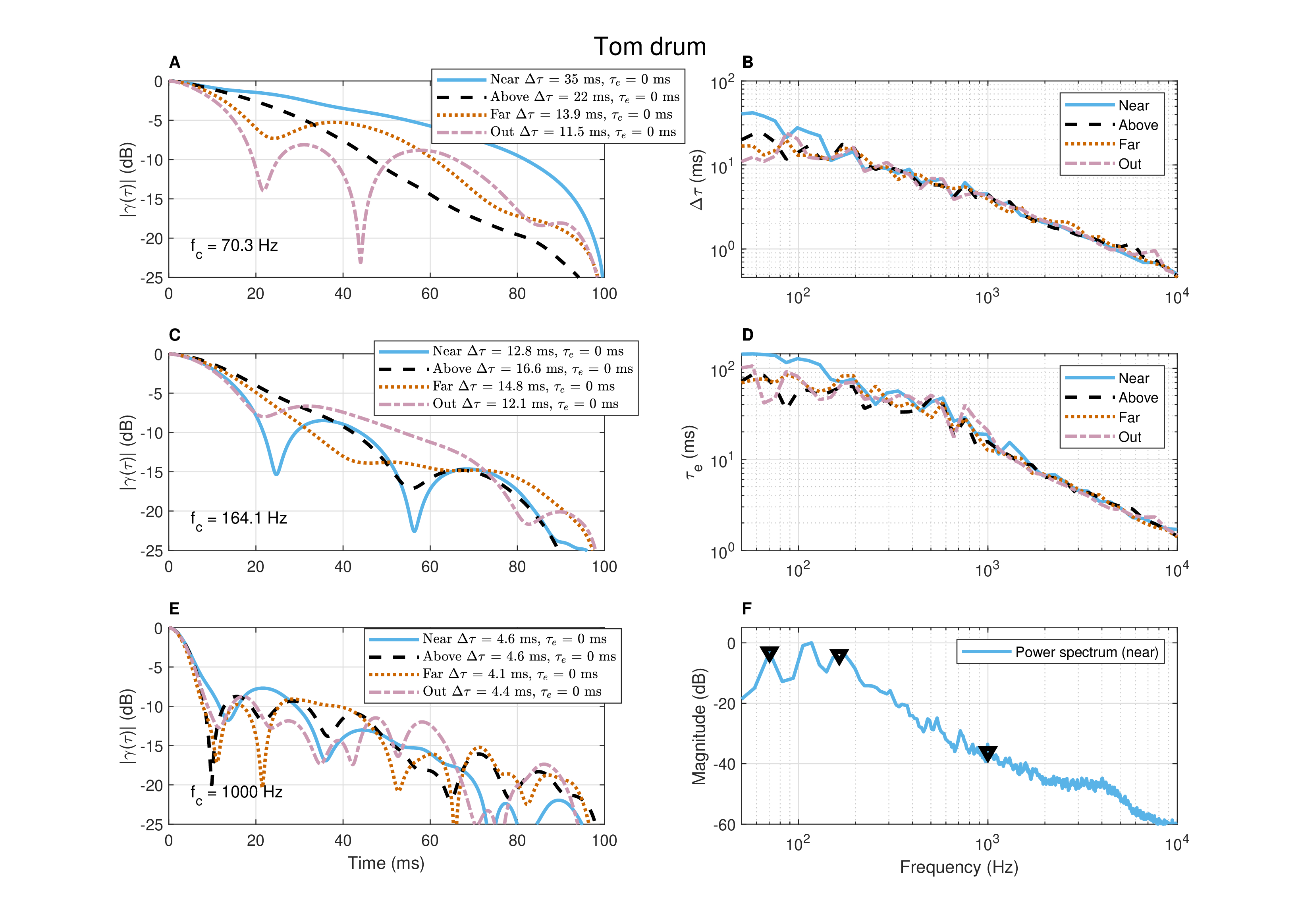
Figure A.8: The autocorrelation of a floor tom drum of a drum set being played for 3 s. The autocorrelation function envelopes of the same material recorded in four different positions in the room are compared at three different frequencies. The first at 70 Hz (plot A) and second at 164 Hz (C) are resonances of the drum, as is marked in the spectrum of the near position (plot F). At 1000 Hz (plot E) and in general above 200 Hz, there are no special spectral features and the sound may be largely incoherent at the source. Plots B and D are the frequency-dependent mean coherence time (at -10 dB) and median running coherence time, or effective duration, respectively.
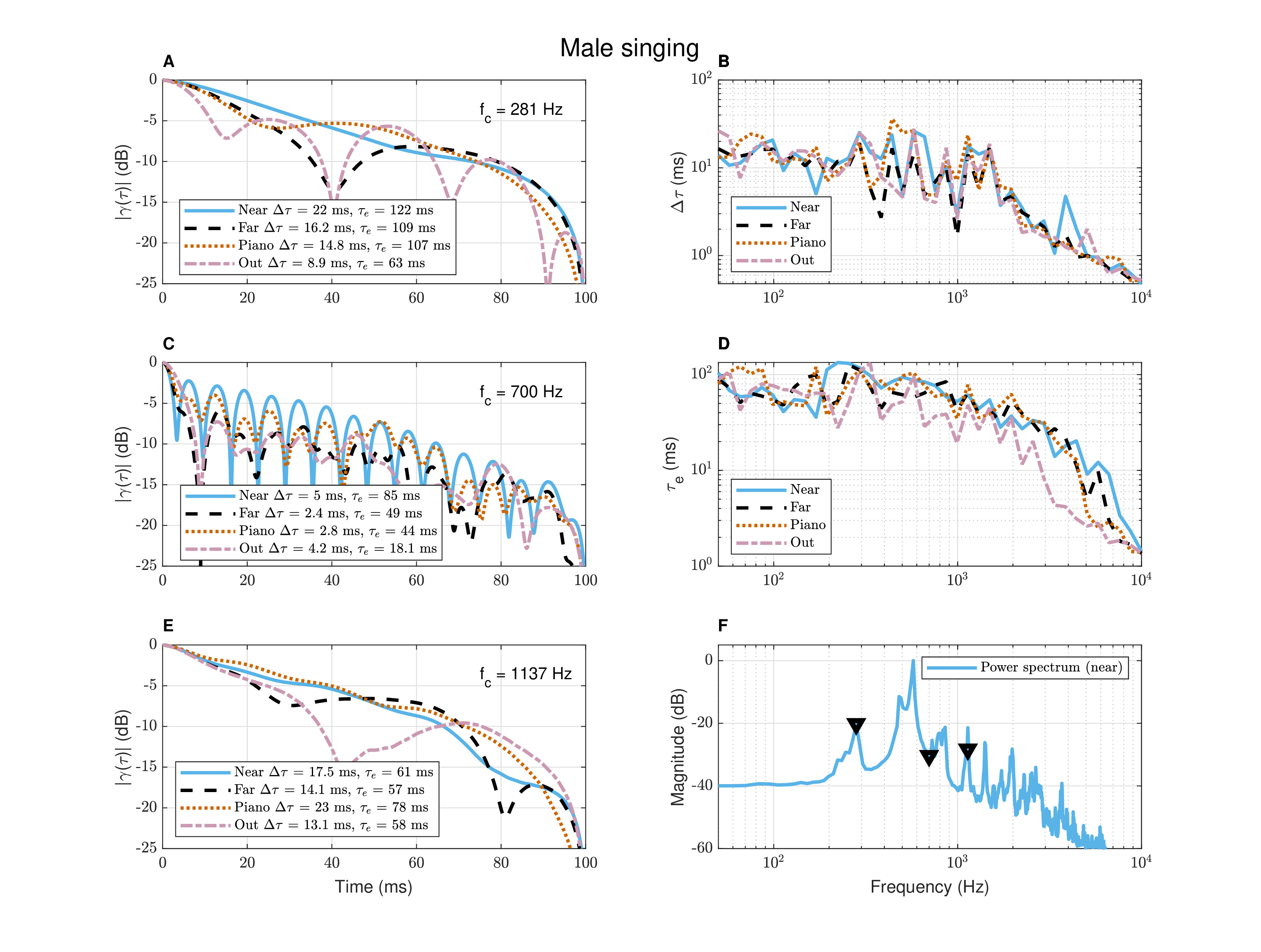
Figure A.9: Autocorrelation of male singing for 1.4 s. The autocorrelation function envelopes of the same material recorded simultaneously in four different positions in the room is compared at three different frequencies. The first at 281 Hz (plot A) is \(f_0\) and the third at 1137 Hz (plot E) is a distinct resonance. The 700 Hz frequency (plot C) was chosen to illustrate the effect of no discernible resonance and low energy on the autocorrelation. The frequencies are marked in the spectrum (plot F). Plots B and D are the frequency-dependent mean coherence time (at -10 dB) and median running coherence time, or effective duration, respectively.
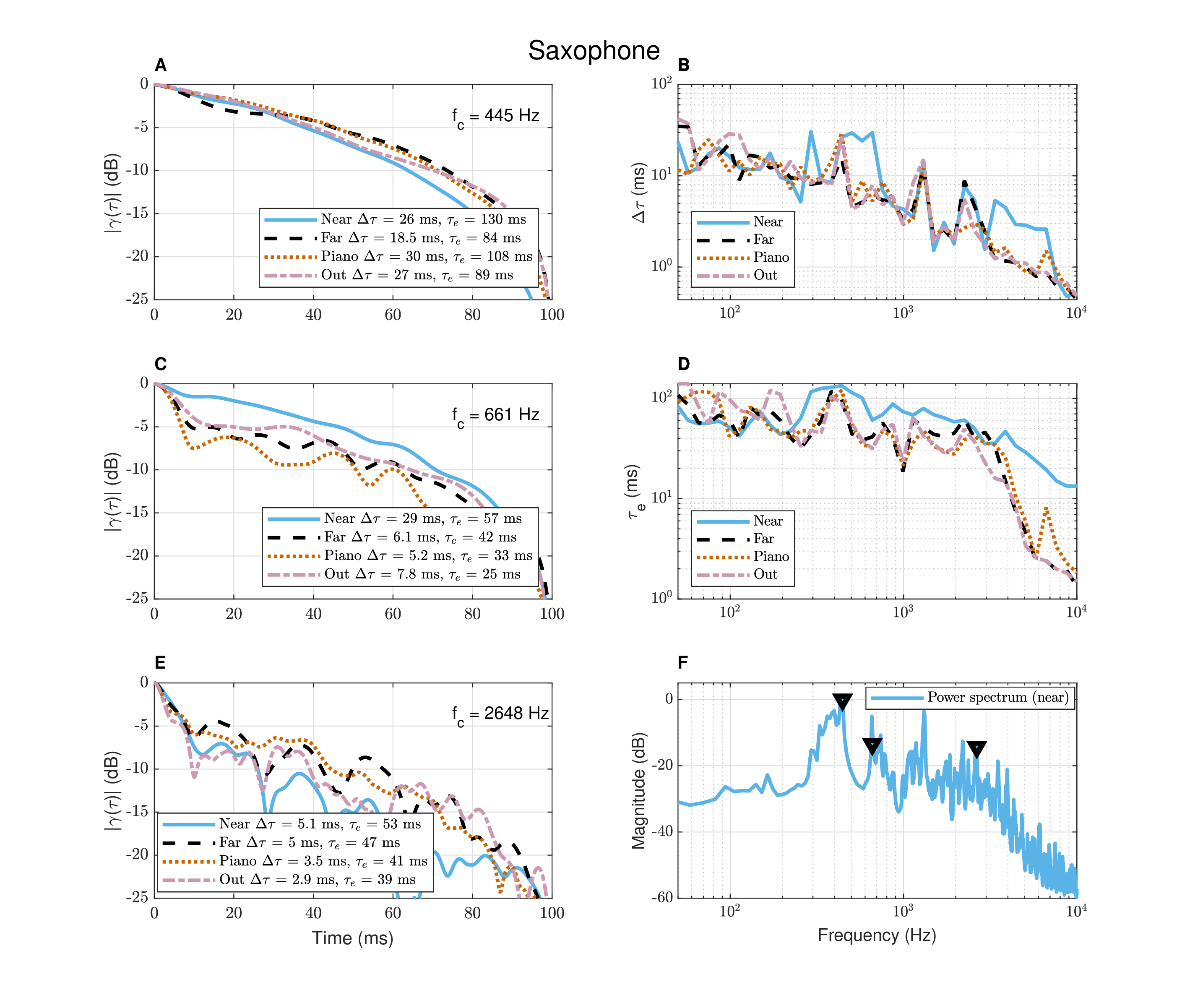
Figure A.10: Autocorrelation of tenor saxophone playing fast notes for 3 s, in the same conditions as the male singing example from Figure §A.9. The frequencies in the analysis (plots A, C, E) were selected from peaks in the spectrum (plot F), but the near position tended to exhibit longer coherence time (plot B) and effective duration (D) than the other microphone positions.
In the second example (Figure §A.9), male singing for 1.4 s is analyzed. Once again, the coherence time estimates were generally longer for the near position both at low frequencies below 150 Hz, and around a couple of distinct resonances (plot B). While the tendency for the coherence time to get shorter with higher frequencies is apparent here too, the additional energy in other spectral components makes the frequency dependence more erratic. This may be gathered by inspecting the second frequency (700 Hz), which was analyzed because it does not correspond to any clear peak. The coherence time at 700 Hz drops significantly to around 5 ms in the near position, or shorter in other positions (plot C). It is lower than the next resonance at 1137 Hz, which has 13–23 ms coherence time, depending on the positions (plot E). The different nature of this source coherence is evident in the variation of the coherence time and effective duration in frequency (plots B and D), which are not nearly as monotonically linear as that of the tom drum.
In the third example (Figure §A.10), a short passage (3 s) of tenor saxophone fast notes was recorded in an identical setup to the singing. While the near-field recording has the longest coherence time, the rank order of the other recordings from the room is not always predictable. Especially in the connected room and the piano, there may have been specific room modes or soundboard resonances that enhanced some of the frequencies. In general, even though the notes that were played are short, they still consist of relatively long periodic portions that have high coherence at low frequencies. However, the relatively high coherence manifests primarily in near-field, as can be seen in the coherence time and effective duration curves (plots B and D).
A.6.2 Decoherence as a function of position and frequency
It has been shown that in reverberation the pressure field is decohered between two points with increasing distance and frequency, given that the sound is stationary and represents a perfectly diffuse field (Cook et al., 1955). How relevant is this effect to more realistic sounds that are nonstationary and are not placed within a perfectly diffuse field? Figure §A.11 shows, once again, the tom drum, saxophone, and male singing recordings—each analyzed at the same three frequencies as in §A.6.1. The coherence functions of pairs of recordings are displayed in comparison with the self-coherence (autocorrelation) function in the near position. It can be seen that in none of the cases is there complete (spatial) coherence between the close and any remote microphone, but rather moderate partial coherence (between -10 and -3 dB) over a narrow time interval, which includes the acoustic path delay. According to Eqs. §8.87 and §8.69, at a distance of 0.8 m (the approximate distance between the “near” and “above” microphones according to the their broadband cross-correlation), the coherence of the tom drum at 70 Hz should have been -16 dB (close to the first zero of the sinc function), whereas we obtained -4 dB. At 164 Hz, for that same distance, the sinc function is past its first zero and the coherence is expected to be -9 dB, whereas the obtained value is -5.7 dB. In the case of the saxophone and singing, for a microphone distance of 1–1.5 m, the coherence of the lowest frequencies should have been around -15 dB in both cases, whereas we obtained -5 and -6 dB, respectively. Similar values are obtained from the coherence functions between the far-field microphones.
Another interesting feature is that it is unpredictable which of the three remote positions is the most decohered one with respect to the near position. In one case it is the “far” position (70 Hz, tom), in some cases it is the “out” position of the small room (tom—164 and 1000 Hz; singing—281 and 700 Hz), and in yet other cases the three positions are about equal (singing—1137 Hz; all saxophone frequencies). Such an erratic behavior can be the result of interaction between the coherence function of the source with local modes and reflections, in addition to the different coherence at the source of the three instruments.
All in all, from the small sample of recordings that was tested, the room acoustics in question cannot be considered a true diffuse field, because it indicates that there are extensive frequency ranges of relatively high degree of coherence. Therefore, the pressure fields in these positions may be better described as partially coherent, rather than completely incoherent.
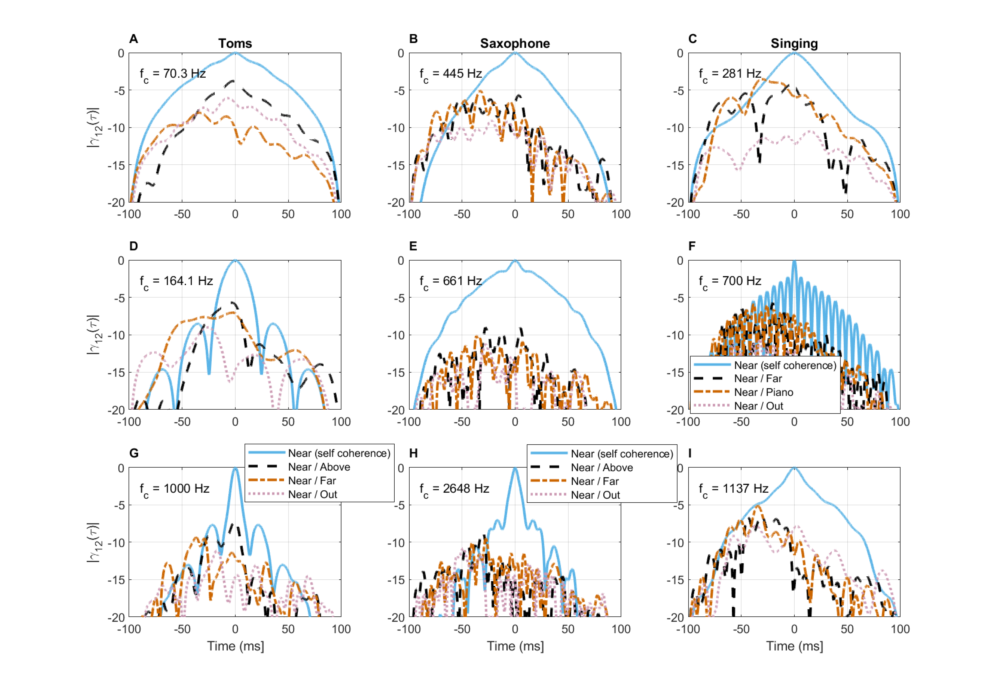
Figure A.11: Cross-correlation of pressure fields in four different positions in the same space for three different sound sources. Each sound source was analyzed around three frequencies, according to Figures §A.8, §A.9, and §A.10.
A.6.3 Cross-spectral coherence
Correlation between frequency components of the pressure field is another effect that was theoretically predicted for diffuse fields (Schroeder, 1962), but has not been demonstrated empirically, to the best knowledge of the author. We demonstrate the effect for the same sound recordings, which we already know did not take place in a perfectly diffuse field. The autocorrelation functions of the (complex) fast Fourier transforms (non-negative frequencies only, 1 Hz resolution) of the broadband pressure fields are plotted in Figure §A.12 for a range of 50 Hz. The data vary in how quickly neighboring frequency components become effectively decorrelated. Borrowing from the previous time-domain analysis, the drop from complete coherence to -3 dB is instantaneous—within \(\Delta f = 1\) Hz. if we treat the -10 dB mark as a rough indicator for incoherence, then a broad range of responses is evident from the plots. In two cases—the “above” tom and `'piano” saxophone positions—the sound barely decoheres over 50 Hz. Other cases can be anything from \(\Delta f\) of 5 to 20 Hz, depending on how the different fluctuations are interpreted. In Schroeder's original paper, \(\Delta f= 3\) Hz for \(T_{60} = 1\) s led to a drop in coherence below -10 dB (Schroeder, 1962; Figure 3).
As larger frequency deviations than predicted by stationary coherence theory were obtained for the present examples, we can conclude that adjacent components are partially coherent, albeit weakly. This supports the general theory of nonstationary coherence, as was briefly reviewed in §8.2.9, which explicitly discusses coherence between different frequency components—something that violates the stationarity assumption in standard coherence theory (Eq. §8.29).
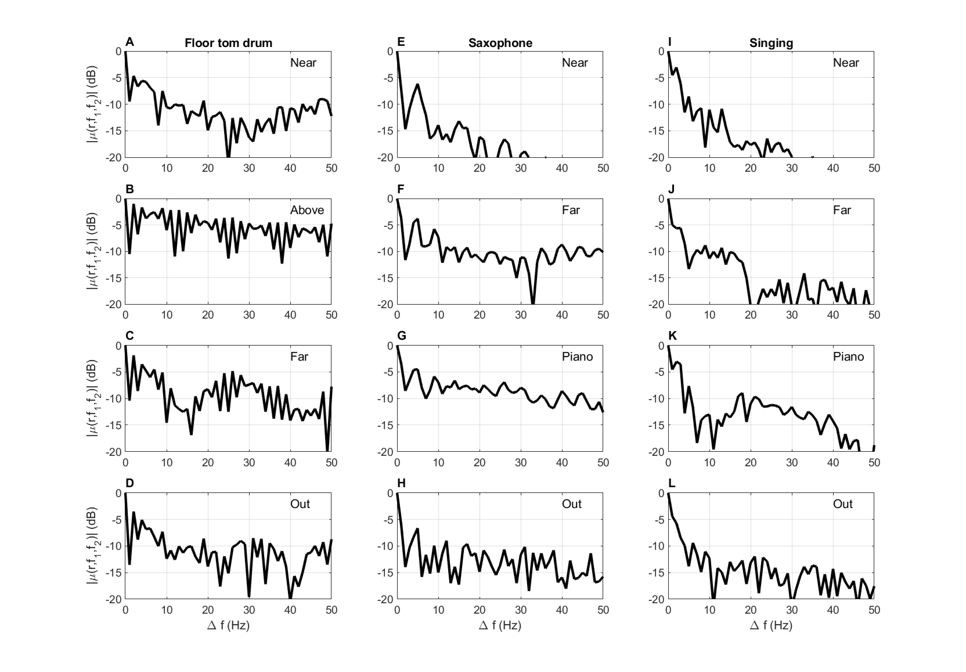
Figure A.12: The autocorrelation of the pressure frequency response of three sources in four different positions in space. See §A.6.1 for further details about the sources and recording positions.
A.7 Conclusion
This appendix presented the coherence functions of a small sample of real acoustic sources that were recorded indoors in different room acoustical conditions. The range of responses is wide and so are the values that are obtained from them. The correspondence between the theoretical results, which are based on the approximate diffuse room acoustics, to the present ones is not always predictable and is made more difficult because of nonstationarity. Still, these results demonstrate the applicability of the concept of partial coherence, either as a descriptor of the narrowband self-coherence of a sound, or of the spatial coherence between difference receiver positions.
The collection of coherence functions above is by no means a representative sample of acoustic sources in general. However, given the dearth of published data about it in the literature, it provides a starting point for more comprehensive attempts to chart this large territory in the future.
Footnotes
179. The coherence time is defined as the measured at the half-maximum point of the main lobe, whereas the effective duration is measured when the function drops to -10 dB. However, the latter is evaluated through extrapolation from -5 dB. See §A.5 and §8.3 for further details.
180. A xylophone-like instrument with tuned metallic bars that produce tones of sharp attack and long sustain. The sound is produced with soft mallets.
181. The largest drum of the drum set, except for the bass drum.
References
Ando, Yoichi. Concert Hall Acoustics. Springer-Verlag, Berlin, Germany, 1st edition, 1985.
Ando, Yoichi, Okano, Toshiyuki, and Takezoe, Yoshitaka. The running autocorrelation function of different music signals relating to preferred temporal parameters of sound fields. The Journal of the Acoustical Society of America, 86 (2): 644–649, 1989.
Bachorowski, Jo-Anne, Smoski, Moria J, and Owren, Michael J. The acoustic features of human laughter. The Journal of the Acoustical Society of America, 110 (3): 1581–1597, 2001.
Cook, Richard K, Waterhouse, RV, Berendt, RD, Edelman, Seymour, and Thompson Jr, MC. Measurement of correlation coefficients in reverberant sound fields. The Journal of the Acoustical Society of America, 27 (6): 1072–1077, 1955.
D'Orazio, Dario, De Cesaris, Simona, and Garai, Massimo. A comparison of methods to compute the "effective duration" of the autocorrelation function and an alternative proposal. The Journal of the Acoustical Society of America, 130 (4): 1954–1961, 2011.
Fletcher, Neville H and Rossing, Thomas D. The physics of musical instruments. Springer Science+Business Media New York, 2nd edition, 1998.
Glasberg, Brian R and Moore, Brian CJ. Derivation of auditory filter shapes from notched-noise data. Hearing Research, 47 (1-2): 103–138, 1990.
Irino, Toshio and Patterson, Roy D. A time-domain, level-dependent auditory filter: The gammachirp. The Journal of the Acoustical Society of America, 101 (1): 412–419, 1997.
Jacobsen, Finn and Nielsen, TG. Spatial correlation and coherence in a reverberant sound field. Journal of Sound and Vibration, 118 (1): 175–180, 1987.
Kapilow, David, Stylianou, Yannis, and Schroeter, Juergen. Detection of non-stationarity in speech signals and its application to time-scaling. In Sixth European Conference on Speech Communication and Technology (EUROSPEECH'99), pages 2307–2310, 1999.
Lentz, Jennifer J and Leek, Marjorie R. Psychophysical estimates of cochlear phase response: Masking by harmonic complexes. Journal of the Association for Research in Otolaryngology, 2 (4): 408–422, 2001.
Patterson, RD, Nimmo-Smith, Ian, Holdsworth, John, and Rice, Peter. An efficient auditory filterbank based on the gammatone function. In Meeting of the IOC Speech Group on Auditory Modelling at RSRE, December 14-15, 1987.
Schroeder, Manfred Robert. Frequency-correlation functions of frequency responses in rooms. The Journal of the Acoustical Society of America, 34 (12): 1819–1823, 1962.
Van Der Ziel, Aldert. On the noise spectra of semi-conductor noise and of flicker effect. Physica, 16 (4): 359–372, 1950.
Voss, Richard F and Clarke, John. '1/f noise' in music and speech. Nature, 258 (5533): 317–318, 1975.
Blinchikoff, Herman J. and Zverev, Anatol I. Filtering in the time and frequency domains. Scitech Publishing Inc., Rayleigh, NC, 2001.