 )
)Chapter 4
Optical imaging
4.1 Introduction
Visual sensation critically depends on the optics of the eye that constitutes an imaging system. This connection implies that different concepts pertaining to the optics of image formation and its quality are deeply ingrained within our visual perception. In turn, it suggests that the study of imaging can be both intuitive and palpable. It was argued in §1.4 that the various auditory image models in literature provide an incomplete analogy to the visual image. These models are mute with respect to some of the most powerful concepts of the optical image such as focus, sharpness, blur, depth of field, and aberrations. In most cases, it is not even clear what the object of the putative auditory image is. This chapter provides a general and selective overview of optical imaging theory, in order to be able to establish a rigorous analogy to the auditory image later in this work. The proposed auditory image will be amenable to the derivation of mathematically and conceptually analogous candidates for almost every aspect of imaging that vision has38. Ideally, some of the intuition from the optical image formation theory can then be translated to hearing as well.
A very brief introduction to spatial optics is given in the next section, where different but complementary analytic frameworks to understand the imaging process are highlighted based on geometrical, wave, and Fourier optics. Then, a simple account of the eye as an optical imaging system is presented. Finally, some links between imaging optics and acoustics and noted.
Readers who are well-versed in imaging optics may comfortably skip this chapter, which is mainly intended for acoustics and hearing specialists with no background in optics. There are numerous introductory texts that cover the topics mentioned below in great depth. The overview is primarily based on general introductory texts on physical optics by Lipson et al. (2010) and Hecht (2017), Fourier optics by Goodman (2017), lasers by Siegman (1986), geometrical optics by Ray (1988) and Katz (2002), and on the comprehensive text by Born et al. (2003).
4.2 Optical imaging theory
Light is the narrow portion of the electromagnetic spectrum that can be detected by human vision in the wavelength range of 400–700 nm and frequency range of 430–750 (THz). This spectral range constitutes a significant portion of the electromagnetic radiation from the sun. It is exploited by many animals as it is biologically stable and detecting it does not suffer from high internal physiological noise (Soffer and Lynch, 1999). Optics is the physical science that deals with light and visible phenomena, but many of its methods are applicable to electromagnetic and scalar wave fields in general.
In daylight, broadband light from the sun is reflected in all directions by objects in the environment. In every point in space, we can place an optical imaging system and obtain an image of a part of the environment, by manipulating the reflected light waves that impinge on it. However, without meeting certain necessary conditions, all that is obtained of other objects are patterns of shadows and light: no image of a tree will spontaneously appear on an adjacent wall—only its shadow.
Let us first define the ideal image \(I_1\), which appears on a plane at a certain distance \(z\) away from the object \(I_0\), as measured along the z-axis, which is referred to as the optical axis. The object and image are referenced to their own parallel rectangular axes \((x,y,z)\) and \((x',y',z')\), respectively. We examine a three-dimensional object that is positioned perpendicular to the optical axis and is described as a light intensity pattern in the X-Y plane with depth along \(z\), \(I_0(x,y,z)\). The ideal image is then (Goodman, 2017; pp. 43–73)
| \[ I_1(x',y',z') = \frac{1}{\left|M\right|}I_0\left(\frac{x}{M},\frac{y}{M} ,\frac{z}{M} \right) \] | (4.1) |
where \(M\) is a constant scaling factor, which entails magnification for \(M>1\) and demagnification for \(M<1\). Thus, an image is a linearly-scaled version of the object in space, also measured as a light intensity pattern. In other words, the image is geometrically similar to the object (see also Born et al., 2003; pp. 152–157). Often, the projection of the object is all that we care about, so both object and image are treated as two-dimensional and perpendicular to the optical axis.
Different theoretical frameworks exist that can account for image formation. We introduce below the two that will be most relevant to the temporal auditory imaging theory.
4.2.1 Geometrical optics
Geometrical optics provides a relatively intuitive framework for analyzing optical systems. It is valid in the limit of infinitesimally small wavelengths, which is often adequate to fully account for the behavior of many important optical instruments (Born et al., 2003; pp. 116–285).
In geometrical optics, light propagates in “rays”, which are normal to the geometrical wavefront of the light arriving from the object. Normally, both spherical and plane waves are considered in the analysis, although local propagation is approximated as plane waves. The space is completely described by the refractive index \(n\), which encapsulates the speed of light at the medium of \(c/n\), where in vacuum and air \(n=1\) and \(c\) is the speed of light. Most geometrical systems of interest describe isotropic and homogenous regions of the medium, in which \(n\) is constant, except for abrupt boundaries where the ray changes direction due to refraction. Critically, we are interested in Gaussian optics, which considers only small angles subtended by the system—the angles that the rays form with respect to the optical axis. This is the paraxial approximation, which leads to simplifying conditions of \(\sin\theta \approx \tan\theta \approx \theta\) and \(\cos \theta \approx 1\).
The simplest system that can produce an image is called a pinhole camera (Hecht, 2017; p. 229), or a camera obscura—referring to its original incarnation as a light-tight room with a small hole in one of its walls that allows for sunlight to enter (Renner, 2009). It comprises three elements that are common in all imaging systems: a pinhole aperture, a darkened compartment, and a screen (see Figure 4.1). The role of the pinhole aperture is to limit the angular extent of light that arrives directly from the object. For an infinitesimally small aperture, every point of the object is mapped to a point-sized sharp region on the screen, which is positioned on the imaged plane. But a very small aperture may reduce the amount of energy too much, so that the image brightness suffers. A large aperture produces brighter images, but allows multiple paths between object points to the screen. The effect is to (geometrically) blur the resultant image, so that fine details of the object cannot be discerned. The darkened compartment is necessary to block all ambient light that can wash out the image. The image that is formed on the screen is scaled by a magnification factor that is determined by the ratio of the distances from the object to the aperture and from there to the screen.
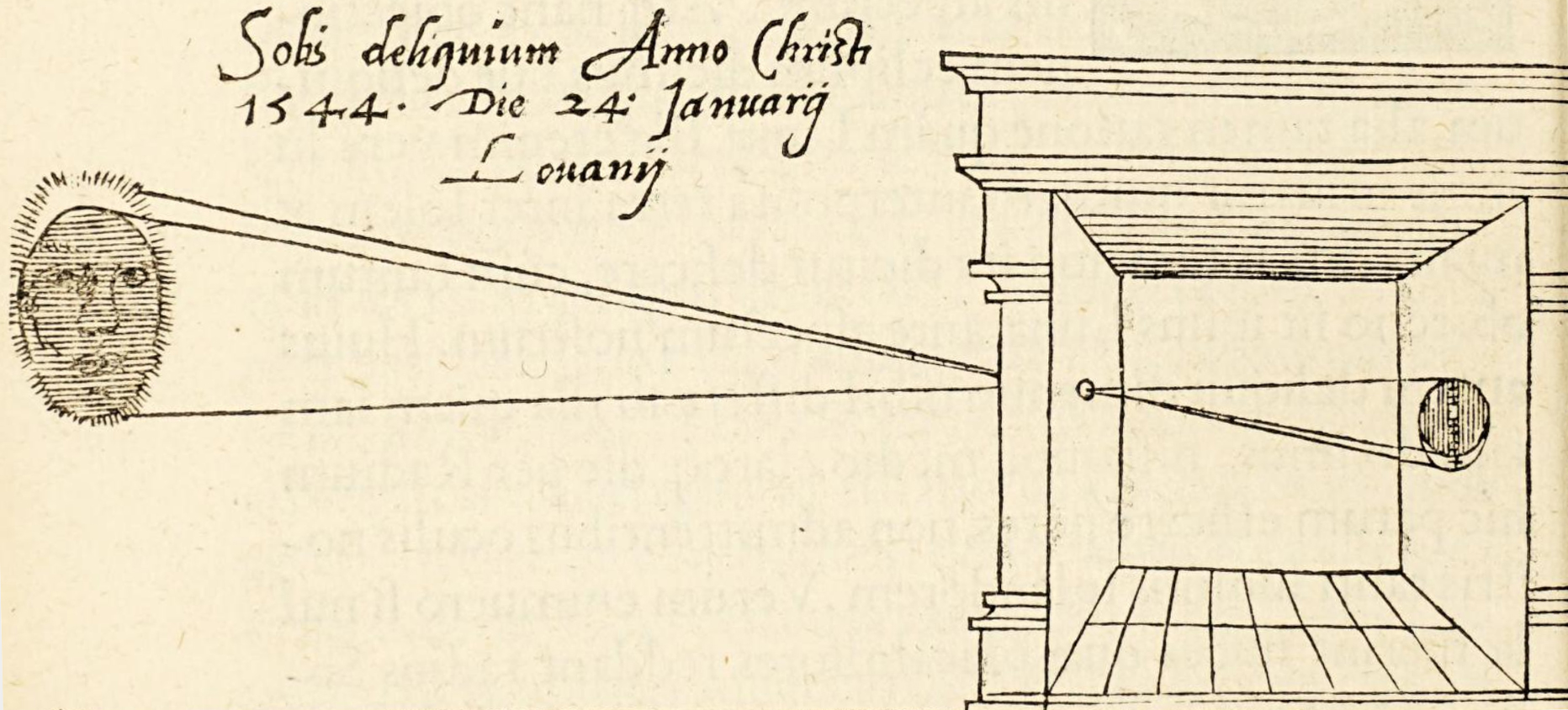
Figure 4.1: The simplest optical imaging system is the camera obscura. The illustration is taken from Frisius (1545, Cap. XVIII, p. 31).
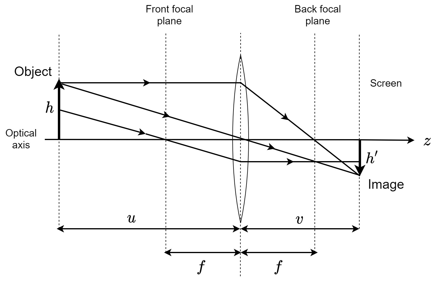
Figure 4.2: A single-lens imaging system. The image of an object of height \(h\) perpendicular to the optical axis is imaged by a thin lens with focus \(f\). The image height \(h'\) is scaled by a magnification factor \(M = -v/u\), where \(u\) is the distance from the object to the lens and \(v\) is the distance from the lens to the image.
An improved design over the pinhole camera is the single-lens camera, which places a thin lens in front of the aperture (Katz, 2002; pp. 223–228) (Figure 4.2). The lens is made from a dense optical material, which has a higher refractive index \(n\) than the surrounding medium. An ideal thin spherical lens is defined by its radii of curvature, \(R_1\) and \(R_2\), and its refractive index, according to the lens-makers' formula (assuming air to be the surrounding medium)
| \[ \frac{1}{f} = (n - 1)\left( {\frac{1}{{R_1 }} - \frac{1}{{R_2 }}}\right) \] | (4.2) |
where \(f\) is the focal length of the lens, measured along the z-axis. The main property of the lens is its ability to transform a beam of light that is parallel to the axis (a plane-wave front that corresponds to an infinitely distant object) to a spherical wavefront that converges at the focus of the lens. Also, parallel rays that are oblique with respect to the optical axis converge to the same point in the focal plane of the lens. The converging property of the lens (for positive lenses with \(f>0\)) makes it suitable to use with larger apertures than are admissible in the pinhole camera, by correcting for the geometrical blur that would have been formed without it. This is expressed through the imaging condition, which ties the object and lens distance \(u\) and the lens and image distance \(v\) to the focal length
| \[ \frac{1}{u} + \frac{1}{v} = \frac{1}{f} \] | (4.3) |
The ratio between the object size (or height) and the image is the magnification, which is given by the distance ratio \(M = -v/u\) (when the distances are both positive), as in the pinhole camera. A negative value of \(M\) implies that the image is inverted.
This simple imaging description breaks down under several conditions. First, real lenses are thick—they have a non-negligible width—which has to be taken into account in the analysis (Born et al., 2003; pp. 171–175). Second, light rays at large angles that violate the paraxial approximation would not converge in the same point as is predicted by the spherical thin lens (Born et al., 2003; pp. 178–180). This deviation from paraxial conditions can increase the likelihood of different distortions and blur in the image, which are variably referred to as aberrations. For example, if a lens has a spherical aberration, then parallel rays arriving from different regions of the lens do not all meet in one focus, but are distributed around it on the optical axis, which makes the image appear blurry. However, the aberrations may be tolerable for the resolution or degree of spatial detail that is required by the system. When using more complex systems with several lenses, it is possible to optimize the image by compensating for some of the aberrations, or trading them off with one another (Mahajan, 2011).
In some cases, the broadband nature of light can become apparent due to the dispersion of light in different media. Dispersion is dependence of the phase velocity on frequency (see §3.2), which is expressed as measurable differences in the refractive index in the entire spectrum covered. If left uncorrected, dispersion may lead to noticeable chromatic aberration, whereby images of different wavelengths (colors) appear at somewhat different distances from the lens (Born et al., 2003; pp. 186–189). In the extreme, a glass prism introduces enough dispersion to spectrally decompose white (or any broadband) light into all of its constituent wavelengths, so that each one refracts in a slightly different direction.
The smallest constriction in the system is called the aperture stop and it controls the amount of light power that is available for imaging. Together with the focal length of the lens, the aperture stop determines the light power per unit area on the imaging plane. This is expressed with the f-number of the system, which is defined as
| \[ f^{\#} = \frac{f}{D} \] | (4.4) |
Where \(D\) is the aperture size (i.e., its diameter). The f-number is the reciprocal of the relative aperture. It expresses the available light power as a unitless number, which enables comparison across different lenses and optical systems, also with more complex designs than the single-lens camera.
It is sometimes useful to define a range of object distances for which the image obtained can be considered sharp. This range is called the depth of field of the system (see Figure 4.3) (Ray, 1988; pp. 180–193). For a system set to sharp focus, the depth of field can be approximated geometrically with
| \[ \mathop{\mathrm{Depth}}\,\mathop{\mathrm{of}}\,\mathop{\mathrm{Field}} \approx \frac{2u^2 f^2 f^{\#} C}{f^4 - {f^{\#}}^2 u^2 C^2 } \approx \frac{2u^2 f^{\#} C}{f^2} \] | (4.5) |
which is measured in units of length, and \(C\) is called the circle of confusion—a limit to the size of the finest detail that is of practical interest in the image. As can be seen, the depth of field is strongly dominated by the distance of the object from the lens \(u\) and by the focal length \(f\). The farther the object is and the smaller the focal length is, the larger the depth of field will be. The depth of field also increases with smaller aperture sizes. The effect of the aperture size can be explained rather intuitively. A system with a large \(f^{\#}\), where \(f \gg D\) implies that the angular extent of light rays that are let into the lens is kept relatively small. This means that there is less light power forming the image, but also that the image is sharper, as information limited to small angles produces less aberrations. If we fix the other parameters in Eq. 4.5, then a high \(f^{\#}\) corresponds to larger depth of field (e.g., Figure 4.3, left). In contrast, when \(D \gg f\) the image is formed by rays arriving at larger angles that make the image blurry quickly away from the focal plane. Images here are much brighter, but they suffer from a shallow depth of field (e.g., Figure 4.3, right). For the effect of the focal length see Figure §15.12.
A complementary concept is the depth of focus, which expresses the tolerance in positioning the screen, on which the image of an object at a given distance would appear sharp. It is approximated as
| \[ \mathop{\mathrm{Depth}}\,\mathop{\mathrm{of}}\,\mathop{\mathrm{Focus}} \approx \frac{2vf^{\#} C}{ f} \approx 2Cf^{\#} \] | (4.6) |
where the second approximation is valid for small magnification systems. Thus, the depth of focus is determined almost exclusively by the relative aperture, with larger aperture causing a reduction in depth of focus.
When an object distance violates the imaging condition (Eq. 4.3) and is well outside of the depth of field of the system, its image suffers a form of blur that is called defocus, which is considered a kind of aberration as well.

Figure 4.3: A demonstration of depth-of-field in still photography. The avocados are in sharp focus in all three photos, whereas the fruit that are nearest and farthest from the lens become gradually more blurry between the photo on the left through to the right, as their depth-of-field decreases. This effect is achieved by fixing the focal length of the camera while increasing the aperture size, as is implied in Eq. 4.4, with f-number values of f/8, f/4, and f/1.4 (left to right) and a lens with focal length of 50 mm.
In reality, the spatial resolution of the image is finite due to diffraction, so that even an infinitesimally small light point on the object would map to a finite disc of light of the image. When the aperture size is very small, the wavelength of the light is no longer negligible as the assumptions of geometrical optics require, in which case the image has to be analyzed using wave theory.
4.2.2 Diffraction and Fourier optics
According to geometrical optics, the pinhole camera should have given an ideal image for an infinitesimally small aperture pinhole size, as long as the illuminating light is bright enough. In reality, the small aperture causes image blur due to diffraction (Young, 1971). In diffraction, wavefronts of different paths sum in amplitude rather than in intensity, as is assumed in geometrical optics. This leads to local constructive and destructive interference patterns that are visible on the image and can severely reduce its quality. Diffraction may be noticeable especially along the edges of the image, which may not appear as sharp as predicted by geometrical optics, but appear as dark and bright fringes (spatial oscillations). In effect, diffraction sets a bound on the achievable image resolution.
Diffraction theory is also based on scalar wave fields, just like geometrical optics, where polarization and electromagnetic effects are neglected39 (Goodman, 2017; pp. 31–61; Born et al., 2003; pp. 412–516). The solution is based on the Huygens-Fresnel principle. It is an extension to Huygens' theorem, which states that40 “Each element of a wave-front may be regarded as the centre of a secondary disturbance which gives rise to spherical wavelets.” Also, “that the position of the wave-front at any later time is the envelope of all such wavelets.” Augustin-Jean Fresnel extended this principle by adding that the secondary wavelets interfere with one another, which he used in his solution for the diffraction problem.
A full solution for the diffraction problem was obtained by Gustav Kirchhoff, who continued from Fresnel, based the homogenous (source-free) Helmholtz wave equation
| \[ (\nabla^2+k^2)E = 0 \] | (4.7) |
where \(E\) is the complex amplitude of the field variable and \(k=2\pi/\lambda\) is its wavenumber. Harmonic time dependence is assumed and factored out. The Kirchhoff-Helmholtz integral is then utilized, which gives a closed expression for the field at an arbitrary point inside a closed boundary on which the field is known. The derivation of the diffraction formula is obtained by summing the amplitudes of all the different optical paths between two points, which have an aperture positioned somewhere between them (Born et al., 2003; pp. 412–430).
The resultant Fresnel-Kirchhoff diffraction formula requires further approximations in order to be usable. We specifically consider the paraxial approximation (Goodman, 2017; pp. 75–114). It coincides with the Fresnel approximation that neglects higher-order terms than quadratic, which nevertheless yields precise results for small angles. In the solution, a planar mask is illuminated by a plane wave field, whose distribution in front of the mask is known. The mask—essentially a geometrical pattern of transparent openings that in imaging can refer to the aperture—is perpendicular to the optical axis (see Figure 4.4). Two solution regimes are obtained—Fresnel diffraction (near-field) and Fraunhofer diffraction (far-field). There are different formulations to the Fresnel diffraction integral, but we refer to the one from Goodman (2017, p. 79), which highlights the resemblance between the two regimes
| \[ E(x,y) = \frac{e^{ikz}}{i\lambda z} e^{\frac{ik}{2z}(x^2+y^2)} \int_{-\infty}^\infty\int_{-\infty}^\infty E(\xi,\eta) e^{\frac{ik}{2z}(\xi^2+\eta^2)} e^{-\frac{2i\pi}{\lambda z}(x\xi + y\eta)} d\xi d\eta \] | (4.8) |
where \(E(\xi,\eta)\) is the complex amplitude of the field on the mask plane, \(\lambda\) is the wavelength of the monochromatic wave, and \(z\) is the distance between the mask and the observer. The double integral sums all the contributions from the mask plane \((\xi,\eta)\) that have optical paths reaching the observer at \((x,y)\). The diffraction is observed as an intensity pattern \(I = EE^* = |E|^2\), which means that the initial quadratic phase factor in Eq. 4.8 cancels out. The presence of the quadratic phase term in the integrand of the Fresnel diffraction integral entails that a closed solution can only be obtained for relatively few problems.
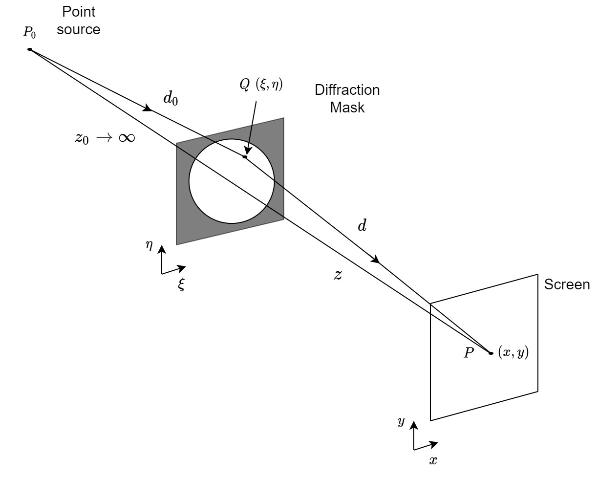
Figure 4.4: The geometry of the Fresnel integral (Eq. 4.8). The source is taken to be very far from the mask, so the light is considered parallel to the optical axis. The illustration is drawn after Figure 7.3 in Lipson et al. (2010).
In the limit of an infinitely far source and observer \(z \gg k(\xi^2+\eta^2)_{max}/2\), so the quadratic phase term in the Fresnel diffraction integral is approximately unity and it simplifies to a special case—the Fraunhofer diffraction
| \[ E(x,y) = \frac{e^{ikz}}{i\lambda z} e^{\frac{ik}{2z}(x^2+y^2)} \int_{-\infty}^\infty\int_{-\infty}^\infty E(\xi,\eta) e^{-\frac{2i\pi}{\lambda z}(x\xi + y\eta)} d\xi d\eta \] | (4.9) |
This integral assumes the form of a scaled two-dimensional Fourier transform of the field \(E(\xi,\eta)\). This opens the door for Fourier analysis and linear system theory, in which the inverse domain corresponds to spatial frequencies that can be used to decompose the field functions41. The spatial frequencies are derived from the propagation vector of the field \(\boldsymbol{\mathbf{k}} = \frac{2\pi}{\lambda}(\alpha \hat{x} + \beta \hat{y} + \gamma \hat{z} )\), where \(\alpha\), \(\beta\), and \(\gamma\) are the direction cosines of \(\boldsymbol{\mathbf{k}}\), so that \(k_x = \alpha/\lambda\) and \(k_y = \beta/\lambda\) are component spatial frequencies. This means that, in this case, the Fourier decomposition is made into component wavefronts that propagate in specific directions with respect to the optical axis. As the wavefront propagates, so does the corresponding angular spectrum in \(k\), which accumulates a component-dependent phase.
The scope of Fresnel diffraction can be generalized for light beam propagation even when no aperture or mask are involved. It is particularly useful in the analysis of lasers beams, which have a Gaussian amplitude profile that can be propagated in closed form. This analysis expresses the field as a traveling wave along the optical axis \(E(x,y,z) = a(x,y,z)e^{-ikz}\), so that \(a(x,y,z)\) is its slowly changing spatial envelope, or essentially, it is the transverse amplitude and phase variation of the beam that is carried over the spatial frequency \(k\). This field can be applied to the homogenous Helmholtz equation by assuming that the change in the beam profile is slow in comparison to the wavelength. The resultant equation is the paraxial Helmholtz equation (Siegman, 1986; pp. 276–279; Goodman, 2017; p. 74)
| \[ \nabla^2 a + 2ik\frac{{\partial a}}{{\partial z}} = 0 \] | (4.10) |
The solution to this equation is a Fresnel integral, which for a Gaussian beam input results in a Gaussian profile as well. This identity between general field propagation and Fresnel diffraction underlines the generality of the concept of diffraction, which was defined by Sommerfeld (quoted in Goodman, 2017; p. 44) as “any deviation of light rays from rectilinear paths which cannot be interpreted as reflection or refraction.”
The thin lens can be analyzed in a manner similar to diffraction as well, if the relative phase delay of the field is computed in different paths (Goodman, 2017; pp. 155-167). The ideal lens converges a parallel wavefront to the a single point in the focal plane. Mathematically, each such wavefront may be mapped to a single spatial component (angle). The thin lens is a phase transformation of the form
| \[ E_1(x,y) = E_0(x,y)\exp\left[-ik\frac{(x^2+y^2)}{2f} \right] \] | (4.11) |
for an input field \(E_0(x,y)\), whose angular extent is smaller than the extent of the lens, so no additional aperture is required. If the lens is smaller than the angular extent of the field, it is necessary to constrain it using a pupil function, which is the aperture associated with the finite extent of the lens. In small angles, the transformation approximately converts plane waves to spherical waves. The spherical wavefront is converging for a positive focus and diverging if it is negative.
In the paraxial approximation of the wave equation, the lens transformation is the (mathematical) dual operation of Fresnel diffraction. The single-lens imaging system can be analyzed by placing a lens between two propagation/diffraction sections. When the imaging condition (Eq. 4.3) is satisfied, all the quadratic phase terms in the integration cancel out, and we are left with a double Fourier transform, which produces the ideal image as in Eq. 4.1 (Goodman, 2017; pp. 168–174). Unlike geometrical optics, the effects of diffraction can now be accounted for when the aperture is small. When it is large, wave theory asymptotically produces the same results as geometrical optics42.
The significance of the aperture in imaging cannot be overestimated. Perhaps the most revealing result from Fourier optics relates the ideal image to the aperture (Goodman, 2017; pp. 185–189). The classical way to think of this problem goes back to Ernst Abbe and later to Lord Rayleigh, who introduced the concepts of entrance pupil and exit pupil—the images of the aperture, as seen from the object and image points of view, respectively (Figure 4.5). Using this approach, the image amplitude can be shown to be the convolution between the ideal image (of geometrical optics, Eq. 4.1) and the point-spread function (the optics jargon for the two-dimensional impulse response) of the aperture, which is the Fraunhofer diffraction pattern of the exit pupil. For a simple pinhole aperture, the pupil effect can be thought of as a filter that removes high spatial-frequency components that subtend the largest angles to the axis and are more likely to contribute to image aberrations (see Figure 4.6). Therefore, designs based on Fourier optics can harness the aperture to process the image in the inverse spatial-frequency domain.
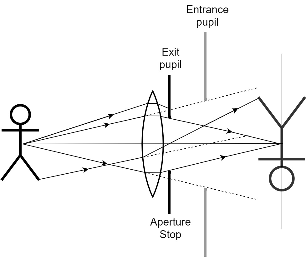
Figure 4.5: Entrance and exit pupils in a simple imaging system with a rear aperture stop that is placed behind the lens. The entrance pupil is the apparent size of the aperture as seen from the object point of view. Therefore, it is the image of the aperture on the side of the lens. The exit pupil is the image of the aperture seen from the image point of view, which in this case is equal to the aperture stop itself. This illustration is a variation on Figure 5.44 in Hecht (2017).
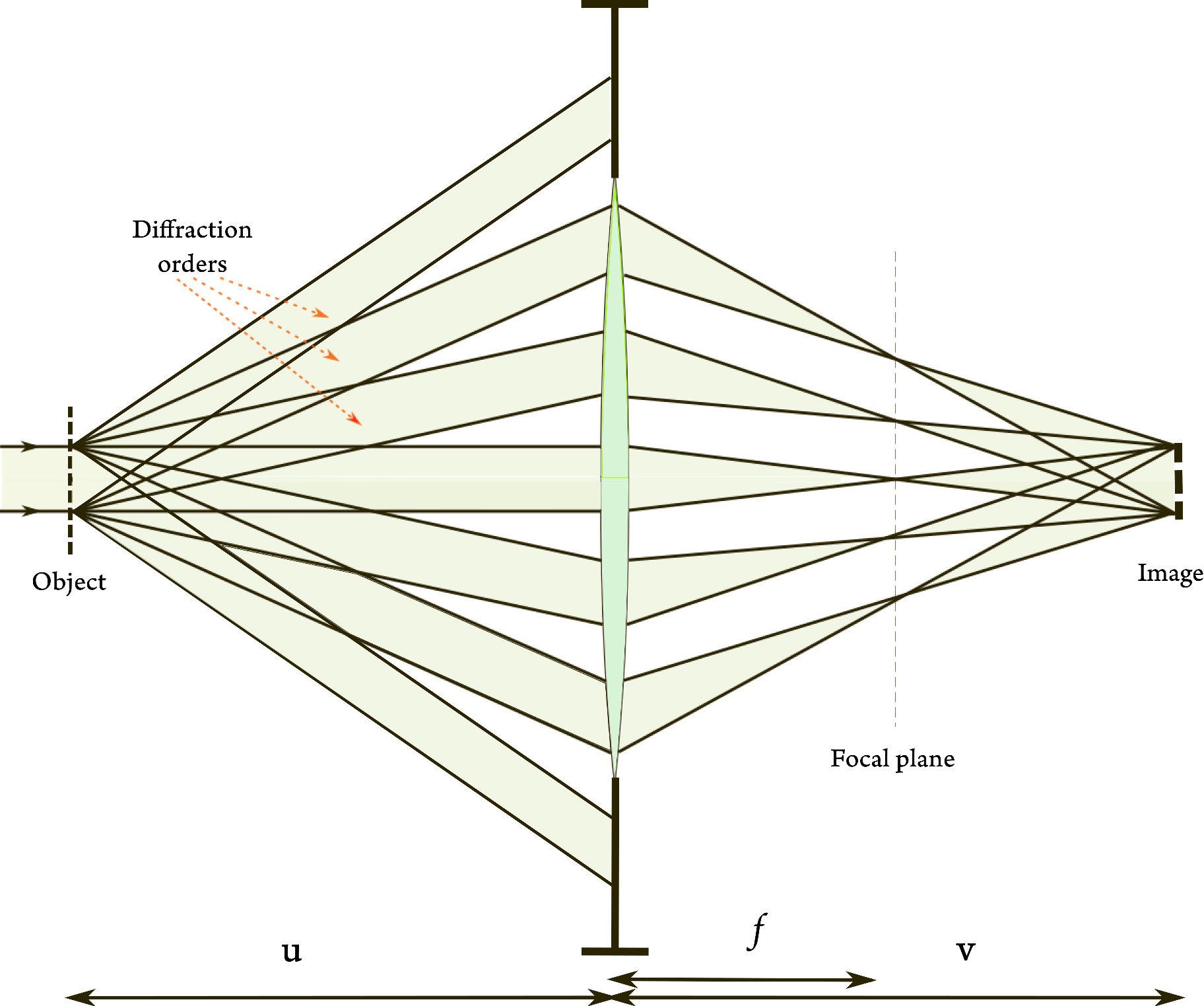
Figure 4.6: Abbe's imaging theory. Light is diffracted from the object, so that different diffraction orders refer to different angles subtended from the optical axis. The lens performs a Fourier-transform-like operation on the light field envelope, so that different angles are mapped to points on the focal plane. From there they continue to the image plane and form the image as an interference pattern between the available diffraction orders. The highest positive and negative orders that are transformed by the lens are cut off by the aperture stop. The illustration is based on Figure 12.3 in Lipson et al. (2010) and on Figure 7.2 in Goodman (2017).
The Fourier representation of imaging as in Figure 4.6 is important in illustrating how every spatial frequency component—one that corresponds to a particular direction of light from the object—is mapped to a particular spatial frequency in the image. This one-to-one mapping takes place at the focal plane when the image is sharp. A blurry image as is caused by defocus or other aberrations is composed from spatial frequencies that are not mapped uniquely to one frequency each, but spread some of their energy to other frequencies at their vicinity. This effectively distorts the spatial representation by not exactly retaining the same spatial pattern, as contours, edges, and other fine details become less well-defined. This is the basis for blur in spatial imaging.
An important example of how the point spread function can be used is to compute the finest details that can be resolved in a diffraction-limited image—an image that does not suffer from any geometrical blurring aberrations. For a circular aperture of diameter \(D\), an object point appears in the image as concentric rings with a fuzzy disc in the image called Airy disc. The Rayleigh criterion sets the minimum resolvable angular detail \(\theta_{min}\) at the first zero of the Airy disc, where a second disc of a second point may be placed to be distinct, and hence resolvable (Lipson et al., 2010; pp. 413–414):
| \[ \theta_{min} = \frac{1.22\lambda}{D} \] | (4.12) |
for a given wavelength \(\lambda\).
4.3 The human eye
Explaining the function of the visual periphery, the eye, becomes trivial, once the basic optical theory of imaging is understood—much unlike the ear. Although the eye does not strictly follow the paraxial approximation, its function is analyzed most regularly using geometrical optics, while allowing for aberrations to account for the realistic image imperfections (Le Grand and El Hage, 1980). The human eye (Figure 4.7) is a wide-angle single-lens imaging system and is similar to a simple camera (Born et al., 2003; pp. 261–263). Objects in front of the eye emit (or rather reflect) light that is focused by the cornea and the crystalline lens of the eye, both of which have a refractive index larger than unity. The lens itself is convergent and aspheric—it has a graduated refractive index between its center and its periphery—which counteracts some of the natural aberrations of the eye. From there, the light refracts through the pupil, which serves as an aperture stop, and into the vitreous humor that has refractive index similar to water. At the focal plane, on the back of the retina, a real upside-down image is formed43. Additional light scattering from the boundaries between the ocular elements within the eye adds relatively little blur to the image (Williams and Hofer, 2003). In daylight conditions and in young healthy eyes, a pupil of about 3 mm in diameter can achieve nearly diffraction-limited imaging, which is almost free of aberrations (Charman, 2010). Refractive errors that cause the focal plane to appear in front (myopia) or behind (hyperopia) the retina are prevalent in the population, but can be optically corrected in many cases using glasses, contact lenses, or a corrective surgery.
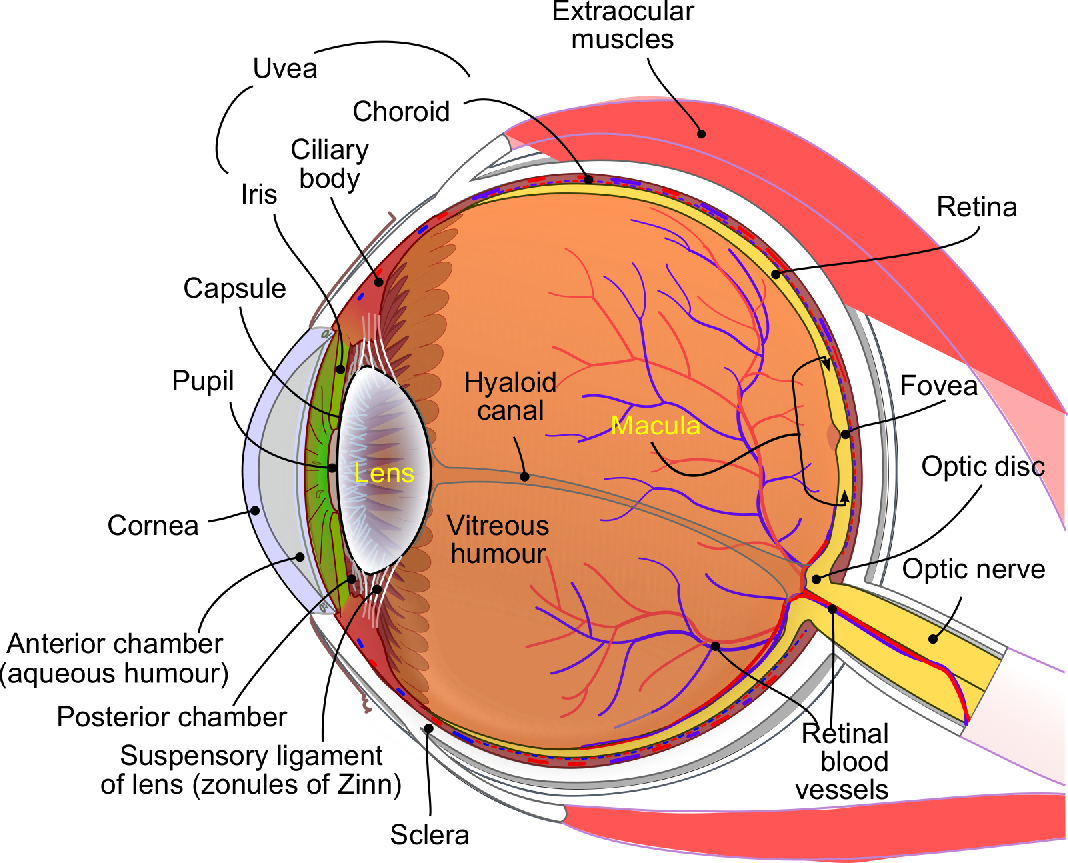
Figure 4.7: The main parts of the human eye (adopted from artwork by Rhcastilhos and Jmarchn, https://commons.wikimedia.org/wiki/File:Schematic_diagram_of_the_human_eye_en.svg).
The retina itself is spherical and is studded with photoreceptors that are directed to the exit pupil and sample the image plane (Charman, 2010). The cones detect narrowband light at moderate and high intensity, which gives sensation to color. The rods are broadband and become dominant only at low light levels. A high density of cone photoreceptors is found at the center of the retina44 in an area called the fovea, which is responsible for the central vision. In the peripheral regions of the retina, the photoreceptors become sparser and more dominated by rods. A network of neurons processes the information from the cones and rods in a convergent fashion (see Figure §1.3), which delivers the neurally coded response to the brain via the optic nerve (Sterling, 2003).
The simple design of the eye is complemented by adaptive mechanisms that are critical for image quality. Three mechanisms enable the eye to control the image quality, which work as a triad, or a reflex—sometimes called the accommodation reflex (Charman, 2008). The first mechanism controls the aperture of the eye, which is the pupil. Its size is controlled by the iris that closes and opens the pupil using annual sphincter and dilator muscles, respectively. In bright illumination conditions, pupil contraction cuts off the high spatial frequencies and increases the apparent depth of field. The second mechanism directly relates to the image sharpness. Ciliary muscles that connect to the lens through tiny ligaments (the zonules of Zinn) control the shape of the eye itself, which modifies its focus and improves the image of objects at different distances in a complex process called accommodation (Toates, 1972; Charman, 2008). The third mechanism is called vergence and is responsible to rotate the eyes inwards and outwards according to the distance of the object. This mechanism is important for the unified binocular perception of the two eyes. The three mechanisms usually work involuntarily, in concert.
Another reflexive feature of the eyes has to do with their movement, which can be either voluntary or involuntary. The eye movement inside its orbit is accomplished by three pairs of muscles. The rapid muscular movements, saccades, scan the scene and are necessary to center the required image on the fovea. During the saccades, vision is suppressed and is activated when the eye is at rest. Further miniature eye movements or microsaccades are continuously present in the eye and, although their role is not entirely clear (Collewijn and Kowler, 2008), visual perception of the image may disappear completely in their absence (Charman, 2010).
The main measure to quantify the visual image quality is called visual acuity and it relates to sharpness—the finest detectable spatial details that can be sensed by the observer (Westheimer, 2010). It is a psychophysical measure, which, to a large degree, is constrained by the periphery. It is maximal in small pupil openings (smaller than 3 mm), which eliminate most aberrations that blur the image and is dictated by the diffraction limit. The best performance that is optically possible in the spatial domain has a spread of 1.5 arcmin or 90 cycles/degree in the spatial frequency domain. These numbers are further constrained by the limited spatial sampling of the cones in the retina, whose average spacing is 0.6 arcmin in the fovea, where they are densest and provide the best resolution.
4.4 Some links between imaging optics and acoustics
The fact that much of the theory in optics relates to scalar effects, where the electromagnetic nature of the wave field is irrelevant, makes many of the results from optics applicable in other wave theories as well. Almost every basic concept from optics was at some point adopted in acoustics, where the scalar pressure field is of highest relevance (see Table §3.1). Geometrical acoustics applies the concepts of sound rays and bases its calculations on intensity only, as phase effects are neglected (Morse and Bolt, 1944; Kinsler et al., 1999; pp. 135–140). Imaging theory is used in ultrasound technologies, as are commonly encountered in medicine (Azhari, 2010). The Kirchhoff-Helmholtz integral that was mentioned as a stepping stone for the diffraction problem solution has found use in wavefield synthesis technology for spatial sound reproduction (Berkhout et al., 1993). Diffraction problems, however, are relatively uncommon in acoustics, which tends to emphasize scattering problems, in which the boundary condition objects are not significantly larger than the wavelength (Morse and Ingard, 1968; pp. 449–463). The results tend to be very complex and are not nearly as influential as those in optics, where the simple effective equivalence between the Fraunhofer diffraction and Fourier transform led to numerous applications.
While both Fourier optics and Fourier acoustics (as applied to auditory signals) are founded on linear system theory and harmonic analysis, they are different in one important respect, which will become clearer over the next two chapters. Acoustic theory generally applies the various transforms as baseband signals, which are real and are calculated from 0 Hz. In contrast, Fourier optics treats its images as bandpass signals. As the optical signals are represented as phasors with slow spatial envelopes carried on a fast traveling wave, the exact carrier frequency is often inconsequential. Thus, the modulation domain in Fourier optics is always complex. Spatial envelopes in auditory signals are of relatively little interest, but temporal envelopes are key. However, they are considered to be real, rather than complex, and are rarely processed using Fourier transforms. We will challenge this convention in acoustics in the chapters to come.
Footnotes
38. The exception are three-dimensional aberrations such as astigmatism and curvature of field, which will not have an obvious analog in hearing.
39. A rigorous analysis that takes into account electromagnetic effects requires much more complex analysis, which yields measurable differences to the scalar theory only close to the edges of the aperture (Born et al., 2003; pp. 633–673).
40. Quoted in Born et al. (2003, p. 141), from Christiaan Huygens' “Treatise on light” (1690), as translated by S. P. Thompson (1912).
41. Fourier optics was pioneered in the 1940s by Pierre-Michel Duffieux (1946 / 1983), but took a couple of decades to properly catch.
42. It should be emphasized that the results of geometrical optics can be rigorously derived from Maxwell's equations and also directly from the scalar wave equation, either for the electric or for the magnetic field, assuming there are no currents or charges in the region. Additionally, this derivation and many others in optics assume harmonic time dependence of the carrier wave—a monochromatic field whose explicit time dependence is usually factored out. Obtaining results for a broader spectrum requires summation or integration of the intensity, as interactions between components are assumed to not take place.
43. Images may be classified as real or virtual. Real images appear on the screen behind the lens, whereas virtual images appear to be in front of the lens to a viewer observing from the behind the lens (Ray, 1988; p. 32). The magnifying glass is the simplest example for a virtual imaging system.
44. The visual axis of the eye does not overlap with the nominal optical axis, which means that the fovea is not located exactly in front of the lens (Charman, 2010).
References
Azhari, Haim. Basics of Biomedical Ultrasound for Engineers. John Wiley & Sons, 2010.
Berkhout, Augustinus J, de Vries, Diemer, and Vogel, Peter. Acoustic control by wave field synthesis. The Journal of the Acoustical Society of America, 93 (5): 2764–2778, 1993.
Born, Max, Wolf, Emil, Bhatia, A. B., Clemmow, P. C., Gabor, D., Stokes, A. R., Taylor, A. M., Wayman, P. A., and Wilcock, W. L. Principles of Optics. Cambridge University Press, 7th (expanded) edition, 2003.
Charman, W Neil. The eye in focus: Accommodation and presbyopia. Clinical and Experimental Optometry, 91 (3): 207–225, 2008.
Charman, Neil. Optics of the eye. In Bass, Michael, Enoch, Jay M., and Lakshminarayanan, Vasudevan, editors, Handbook of Optics. Fundamentals, Techniques, & Design, volume 3, pages 1.1–1.65. McGraw-Hill Companies Inc., 2nd edition, 2010.
Collewijn, Han and Kowler, Eileen. The significance of microsaccades for vision and oculomotor control. Journal of Vision, 8 (14): 20–20, 2008.
Frisius, Gemma. De Radio Astronomico et Geometrico liber. apud Greg. Bontium. Antwerp, 1545.
Goodman, Joseph W. Introduction to Fourier Optics. W. H. Freeman and Company, New York, NY, 4th edition, 2017.
Hecht, Eugene. Optics. Pearson Education Limited, Harlow, England, 5th edition, 2017.
Katz, Milton. Introduction to Geometrical Optics. World Scientific Publishing Co. Pte. Ltd., Singapore, 2002.
Kinsler, Lawrence E, Frey, Austin R, Coppens, Alan B, and Sanders, James V. Fundamentals of Acoustics. John Wiley & Sons, Inc., New York, NY, 4th edition, 1999.
Le Grand, Y. and El Hage, S. G. Physiological Optics. Springer-Verlag Berlin Heidelberg, 1980.
Lipson, Ariel, Lipson, Stephen G, and Lipson, Henry. Optical Physics. Cambridge University Press, 4th edition, 2010.
Mahajan, Virendra N. Aberration Theory Made Simple, volume TT93. SPIE Press, Bellingham, WA, 2nd edition, 2011.
Morse, Philip M. and Ingard, K. Uno. Theoretical Acoustics. Princeton University Press, Princeton, NJ, 1968.
Morse, Philip M and Bolt, Richard H. Sound waves in rooms. Reviews of Modern Physics, 16 (2): 69, 1944.
Ray, Sidney F. Applied Photographic Optics: Imaging Systems for Photography, Film, and Video. Focal Press, London & Boston, 1988.
Renner, Eric. Pinhole Photography: From Historic Technique to Digital Application. Focal Press, Burlington, MA, 4th edition, 2009.
Siegman, Anthony E. Lasers. University Science Books, Mill Valley, CA, 1986.
Soffer, Bernard H and Lynch, David K. Some paradoxes, errors, and resolutions concerning the spectral optimization of human vision. American Journal of Physics, 67 (11): 946–953, 1999.
Sterling, Peter. How retinal circuits optimize the transfer of visual information. In Chalupa, Leo M. and Werner, John S., editors, The Visual Neurosciences, volume 1, pages 234–259. The MIT Press, Cambridge, MA and London, England, 2003.
Toates, FM. Accommodation function of the human eye. Physiological Reviews, 52 (4): 828–863, 1972.
Westheimer, Gerald. Optics of the eye. In Bass, Michael, Enoch, Jay M., and Lakshminarayanan, Vasudevan, editors, Handbook of Optics. Fundamentals, Techniques, & Design, volume 3, pages 4.1–4.17. McGraw-Hill Companies Inc., 2nd edition, 2010.
Williams, David R. and Hofer, Heide. Formation and acquisition of the retinal image. In Chalupa, Leo M. and Werner, John S., editors, The Visual Neurosciences, volume 1, pages 795–810. The MIT Press, Cambridge, MA and London, England, 2003.
Young, M. Pinhole optics. Applied Optics, 10 (12): 2763–2767, 1971.