 )
)Chapter 12
The temporal imaging equations
12.1 Introduction
Having obtained a paraxial-equation analog as well as two distinct dispersive auditory segments separated by a time lens, we are now in a position to put them together and see how they work as a full imaging system. This chapter is therefore dedicated to the presentation of the temporal imaging equations. The equations will be then applied to psychoacoustic data of Schroeder-phase complex thresholds that specifically targeted the cochlear phase curvature, although we reinterpret them as applying to the entire auditory dispersive path. Derived aperture time durations will be compared with direct measurements of temporal window of the chinchilla along with a few more human psychoacoustic temporal window data points.
Using the paratonal equation (§10.21) (originally, the “paraxial” dispersion equation) of Akhmanov et al. (1968), Akhmanov et al. (1969) as a foundation, the analogy to a full spatial imaging system in the temporal domain was made complete by Kolner and Nazarathy (1989). Kolner (1994a) then perfected the solution and elaborated the theory (Kolner, 1994b; Kolner, 1997), and together with colleagues included treatments for aberrations, additional imaging applications, and some alternative configurations to the basic setup (Bennett et al., 1995; Bennett and Kolner, 1999a; Bennett and Kolner, 1999b; Bennett and Kolner, 2000a; Bennett and Kolner, 2000b; Bennett and Kolner, 2001). A very similar analogy to spatial imaging that anticipated their work was suggested earlier by Tournois (1968). Another similar technique using electric signals was also introduced independently by Caputi (1971), where the time lens was replaced with a standard mixer, but did not receive much attention at the time. Aspects of this theory and other applications of the dispersion equation have been successfully applied in many high-end optical systems from the 1990s. Most notably, it is applied in real-time fast optical spectroscopy that can image microscopic events at the femtosecond range. For reviews of principles and applications of the space-time analogy in optics, see Salem et al. (2013), Goda and Jalali (2013), Torres-Company et al. (2011) and Kolner (2011).
12.2 Temporal imaging with a single time lens
The derivation of the temporal imaging equations is based on Kolner (1994a, Section VII), which itself is completely analogous to the standard Fourier optics approach to spatial imaging, as is derived in Goodman (2017, pp. 155-177). Kolner's derivation will be then supplemented with equations that include the effect of defocusing.
The analysis follows the complex envelope of a modulated signal (a pulse) through a first dispersion, into a time lens, and out through a second dispersion, where an image is formed. The modulation is assumed to be narrowband around a constant carrier that will be implicit throughout the analysis—a condition that in the context of hearing we called paratonal. Therefore, while the carrier changes between acoustic, vibrational, compression, mechanical traveling wave, shear motion, ciliary movements, electrical, and neural forms, the information that it carries is assumed to be conserved (§5.2.4). As in §10, the medium absorption (or gain) is taken to be constant in frequency with negligible higher-order terms.
At the origin, an envelope \(a(0,\tau)\) with spectrum \(A(0,\omega)\) is carried by a plane wave carrier through a dispersive medium. Let us define the group-velocity dispersion transformation \(D\) based on the kernel of the solution of the paratonal equation §10.22,
| \[ D (\zeta ,\omega ) = \exp \left( { \frac{{- i \beta”}\zeta \omega ^2}{2} } \right) \] | (12.1) |
The input dispersion in the auditory system was defined by the combined effect of the outer, middle, and inner ears, up to the time lens in the organ of Corti (Eqs. §11.1 and §11.4). Therefore, any reference to \(\beta”\) and \(\zeta\) can be made implicit
| \[ u \equiv \frac{{\beta”_1}\zeta _1}{2} \] | (12.2) |
The first dispersion \(D_1\) is therefore defined as
| \[ D_1 (\zeta _1 ,\omega ) = \exp \left( -iu\omega ^2 \right) \] | (12.3) |
Using \(D_1\), the general inverse-Fourier transform solution of Eq. §10.22 is rewritten to obtain the time-domain envelope at the output of \(D_1\), in the traveling-wave coordinate system
| \[ a(\zeta _1 ,\tau ) = {\cal F}^{ - 1} \left[ {A(0,\omega )D_1 (\zeta _1 ,\omega )} \right] \] | (12.4) |
Following the first dispersion, we would like to add the time lens to the signal path. The effect of the time lens is multiplicative in the time domain (Eq. §10.29) and is
| \[ h_L (\tau) = \exp \left( {\frac{{is\tau ^2 }}{{4}}} \right) \] | (12.5) |
for a lens with curvature \(s = f_T/2\omega_c\), \(f_T\) being the focal time of the time lens, as was identified in the organ of Corti in §11.6.3. The time lens size is not factored in directly in its transfer function, so we take it to be a “thin time lens”, that extends infinitesimally to \(\zeta = \zeta_1+\varepsilon\). The envelope is then multiplied by \(h_L(\tau)\) and becomes
| \[ a(\zeta _1 + \varepsilon ,\tau ) = {\cal F}^{ - 1} \left[ {A(0,\omega )D_1 (\zeta _1 ,\omega )} \right]h_L(\tau ) \] | (12.6) |
and
| \[ A(\zeta _1 + \varepsilon ,\omega ) = \frac{1}{{2\pi }}\left[ {A(0,\omega )D_1 (\zeta _1 ,\omega )} \right] * H_L(\omega ) \] | (12.7) |
where the convolution operation is marked by \(*\) and is applied according to the convolution theorem in the second equality. Behind the lens (where \(\zeta > \zeta_1+\epsilon\)) the wave propagates through second dispersion \(D_2\), which is defined just like in Eq. 12.3, but this time for the neural dispersion, which includes, roughly, the contributions from the inner hair cells, auditory nerve, brainstem, all the way to the inferior colliculus (§11.7.3)
| \[ D_2 (\zeta _2 ,\omega ) = \exp \left( -iv\omega ^2 \right) \] | (12.8) |
This dispersion then multiplies Eq. 12.7, to obtain the frequency-domain transform of the complete path. Applying the inverse Fourier transform on it, the final envelope is then obtained
| \[ a_n(\zeta _2,\tau ) = {\cal F}^{ - 1} \left\{ \left[ \left( \frac{1}{2\pi} A(0,\omega )D_1 (\zeta _1 ,\omega ) \right) * H_L(\omega )\right] D_2 (\zeta _2 ,\omega ) \right\} \] | (12.9) |
where the subscript \(n\) was added to emphasize that the envelope is sampled (or encoded) in the neural domain. This expression can be solved by writing the convolution integral and inverse Fourier transform explicitly, and by changing the order of integration
| \[ a_n(\zeta _2 ,\tau ) = \frac{1}{{4\pi ^2 }}\int_{ - \infty }^\infty {A(0,\omega ')D_1 (\zeta _1 ,\omega ')d\omega '} \int_{ - \infty }^\infty {e^{i\omega \tau } D_2 (\zeta _2 ,\omega )H_L(\omega - \omega ') d\omega} \] | (12.10) |
The lens transfer function \(h(\tau)\) (Eq. 12.5) was Fourier transformed earlier (Eq. §10.33) and is repeated with the time shifted argument of the convolution integral
| \[ H_L(\omega - \omega ') = \sqrt{4\pi is} \exp \left[-is (\omega - \omega ')^2\right] \] | (12.11) |
The second integral in (12.10) can be solved first
| \[ \frac{1}{{2\pi }}\int_{ - \infty }^\infty {D_2 (\zeta _2 ,\omega )H_L(\omega - \omega ')e^{i\omega \tau } d\omega } = \sqrt {\frac{{is}}{\pi }} \int_{ - \infty }^\infty {\exp \left( { - iv\omega ^2 } \right)\exp \left[ { - is(\omega - \omega ')^2 } \right]} e^{i\omega \tau } d\omega \\ = \sqrt {\frac{{is}}{\pi }} \exp ( - is\omega '^2 )\int_{ - \infty }^\infty {\exp \left( { - i(v + s)\omega ^2 } \right)\exp \left[ {i\omega (\tau + 2s\omega ')} \right]} d\omega \\ = \sqrt {\frac{s}{{v + s}}} \exp ( - is\omega '^2 )\exp \left[ {\frac{{i(\tau + 2s\omega ')^2 }}{{4(v + s)}}} \right] \\ \] | (12.12) |
Using this expression back in (12.10), we obtain a closed-form formula for the output temporal envelope, as an integral transform of the input envelope spectrum (Kolner, 1994a):
| \[ a_n(\zeta _2 ,\tau ) = \frac{1}{{2\pi }}\sqrt {\frac{s}{{v + s}}} \exp \left[ {\frac{{i\tau ^2 }}{{4(v + s)}}} \right]\int_{ - \infty }^\infty A(0,\omega ')\exp \left[ { - i\left( {u + s - \frac{{s^2 }}{{v + s}}} \right)\omega '^2 + \frac{is\tau \omega '}{{v + s}}} \right] {d\omega '} \] | (12.13) |
This is essentially a Fourier transform of the input envelope spectrum in a scaled coordinate system after it has been modulated by a quadratic phase term that depends on all three parameters \(u\), \(v\), and \(s\). An additional quadratic phase term modulates the integral and depends only on \(v\) and \(s\). Eq. 12.13 is analogous to the full solution of the spatial imaging system (Goodman, 2017; p. 169, Eq. 6-33), and it belongs to the important family of linear canonical transforms (LCT)—a generalization of Fourier and other integral transforms (see §C).
12.2.1 Ideal temporal imaging
In order to recover the original envelope after the dispersive effect, it is necessary to look for a condition under which the quadratic phase term in the integrand of Eq. 12.13 vanishes, namely,
| \[ u + s - \frac{{s^2 }}{{v + s}} = 0 \] | (12.14) |
which is satisfied when
| \[ \frac{1}{u} + \frac{1}{v} = -\frac{1}{s} \] | (12.15) |
This imaging condition is the temporal analog to the spatial lens law (Eq. §4.3) and is nearly identical functionally, only with opposite signs.
Let us redefine the scaling factor in the inverse Fourier transform of Eq. 12.13 using the magnification \(M\), also in analogy to spatial imaging,
| \[ M\equiv\frac{v+s}{s} \] | (12.16) |
When the temporal imaging condition (Eq. 12.15) is satisfied then the magnification is additionally equal to \(M_0\),
| \[ M_0 = -\frac{v}{u} = M \] | (12.17) |
which is sometimes more convenient to use. Plugging the imaging condition of Eq. 12.15 and the magnification definition in Eq. 12.13, and using the definition of \(s\) (Eq. §10.32) the output transform simplifies to
| \[ a_n (\zeta _2 ,\tau ) = \frac{1}{{2\pi \sqrt M }}\exp \left[ {\frac{{i\omega _0 \tau ^2 }}{{2Mf_T }}} \right]\int_{ - \infty }^\infty {A(0,\omega )\exp \left( {\frac{i\tau \omega}{M}} \right)d\omega } \] | (12.18) |
which is identically equal to
| \[ a_n (\zeta _2 ,\tau ) = \frac{1}{{2\pi \sqrt M }}\exp \left[ {\frac{{i\omega _0 \tau ^2 }}{{2Mf_T }}} \right]a \left( 0,\frac{\tau }{M} \right) \] | (12.19) |
This remarkable result indicates that at the output of the dispersive system, when the imaging condition of Eq. 12.15 is satisfied, a scaled version of the original temporal envelope is obtained. Except for the quadratic phase, this is an ideal image according to the general definition of an image (Eq. §4.1). It becomes exact for intensity imaging for which this global quadratic phase term vanishes. The conditions for which the quadratic phase can be neglected in amplitude imaging will be investigated later in the chapter (§12.6). Once again, this temporal imaging result is completely analogous to the known two-dimensional spatial images (Goodman, 2017; pp. 169–172). An example of this transform on an arbitrary pulse that is scaled by a factor of \(M=2\) is displayed in Figure 12.1 (left). The effect of the quadratic phase can be seen only on the amplitude waveform and not on the envelope. When the narrowband modulated waveform with the carrier is displayed, then the chirping effect of the quadratic phase is made visible (right).
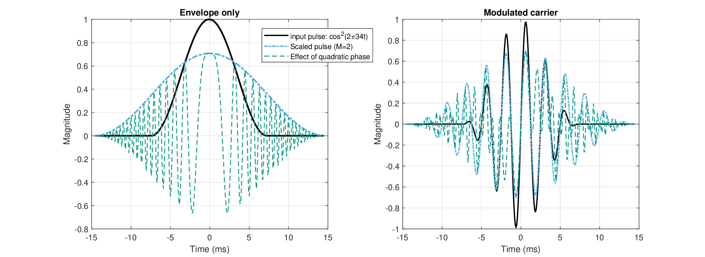
Figure 12.1: An illustration of temporal imaging (Eq. 12.19) for a cosine-squared pulse with: \(f_c=400\) Hz, \(f_{AM}=34\) Hz, \(f_{T}=0.001\,\,\mathop{\mathrm{s}}\), and \(M=2\) (magnification). Left: The initial envelope (narrow pulse), the magnified pulse envelope (wide), and the effect of the quadratic phase on the amplitude (real part only; green dash). Right: The modulated (real) signals before and after imaging, showing the chirping effect of the quadratic phase (in green) and the perfectly imaged unchirped amplitude image (in blue). Only the center-most portion of the pulse is unaffected by the quadratic phase, while the side lobes are corrupted by the global quadratic phase.
12.2.2 Nonideal imaging of a Gaussian pulse
In general, we cannot assume that the imaging condition is satisfied and that the image is in sharp focus. Thus, the full transform of Eq. 12.13 has to be evaluated to obtain the defocused image. A general solution for arbitrary envelopes cannot be obtained for this transform, so the simplest illustration to its effect would be to use a particular envelope—a real (unchirped) Gaussian pulse of width \(t_0\)
| \[ a(0,\tau) = a_0\exp \left(-\frac{\tau^2}{2t_0^2} \right) \] | (12.20) |
The envelope spectrum is given by
| \[ A(0,\omega) = \int_{ - \infty }^\infty a(0,\tau) e^{-i\omega t}dt = \sqrt{2 \pi} a_0 t_0 \exp\left(-\frac{t_0^2 \omega^2}{2} \right) \] | (12.21) |
Plugging it in Eq. 12.13 gives
| \[ a_n(\zeta _2 ,\tau ) = \frac{a_0 t_0}{\sqrt{2 \pi}} \sqrt {\frac{s}{{v + s}}} \exp \left[ {\frac{{i\tau ^2 }}{{4(v + s)}}} \right]\int_{ - \infty }^\infty {d\omega '} \exp \left\{ \left[ \frac{- t_0^2}{2} - i\left( {u + s - \frac{{s^2 }}{{v + s}}} \right) \right]\omega '^2 + {\frac{i s \tau\omega '}{{v + s}} } \right] \] | (12.22) |
Using Siegman's Lemma, the solution to Eq. 12.22 is given by
| \[ a_n(\zeta _2 ,\tau ) = a_0 t_0 \sqrt{ \frac{\frac{s}{v + s}}{2 \left[ \frac{t_0^2}{2} + i\left( {u + \frac{{vs }}{{v + s}}} \right) \right]}} \exp \left[ {\frac{{i\tau ^2 }}{{4(v + s)}}} \right] \exp \left\{ \frac{-\left(\frac{s}{{v + s}}\tau\right)^2}{ 4\left[ \frac{t_0^2}{2} + i\left( {u + \frac{{vs }}{{v + s}}} \right) \right]} \right\} \] | (12.23) |
which reduces to the form of Eq. 12.19, if the imaging condition is satisfied, so the imaginary term in the denominator of the second exponent and in the square root becomes zero. However, if the imaging condition is not satisfied, then the magnification factor cannot be completely separated from the pulse width itself, which results in an effective pulse broadening and chirping. We can define a new complex width \(t'_1\) for the output
| \[ t'_1 = \frac{\sqrt{ t_0^2 + 2i\left( u + \frac{vs }{v + s} \right) }}{\frac{s}{v+s}} = t_0 M\sqrt{ 1 + \frac{2i}{t_0^2}\left( u + \frac{vs }{v + s} \right) } = M't_0 \] | (12.24) |
where we also defined a new magnification factor \(M'\), which is a complex function of the input width and the parameters of the system, including \(M\),
| \[ M' = M\sqrt{ 1 + \frac{2i}{t_0^2}\left( u + \frac{vs }{v + s} \right) } \] | (12.25) |
The imaginary part of \(M'\) results in chirping that may be undesirable in imaging. It can be reduced by minimizing the imaginary term under the radical in Eq. 12.25, which can be rewritten
| \[ 2i\left(u + \frac{vs }{v + s} \right) = \frac{2i}{v}\left(\frac{1}{M} - \frac{1}{M_0} \right) \,\,\,\,\,\,\,\,\, v \neq 0 \] | (12.26) |
using the definitions of \(M\) and \(M_0\) (Eqs. 12.16 and 12.17). Therefore, \(M=M_0\) only in ideal imaging, which also does not chirp.
Finally, the output pulse of Eq. 12.23 can be written more compactly using the definition of \(M'\), in a similar form to the ideal image
| \[ a_n(\zeta _2 ,\tau ) = \frac{a_0}{\sqrt{M'}} \exp \left[ {\frac{{i\tau ^2 }}{{4(v + s)}}} \right] \exp\left[-\frac{1}{2}\left(\frac{\tau}{M't_0}\right)^2\right] \] | (12.27) |
Although specific to a Gaussian input, this expression is almost of the same form as Eq. 12.19. As will turn out in the next section, this solution is more relevant to the auditory system than the ideal imaging transform. The implications of having a defocused imaging will be explored in depth later in this work.
Although realistic signals are not limited to pulses, the system (mainly the time lens) can process only a limited extent of duration of every object. This is analogous to the spatial angle that an object occupies with respect to a camera lens, so it may still be fitted on a single image. In audio signal processing this is achieved with a window function, which is called an aperture in optics. The existence of an aperture in the auditory system will arise organically through the analysis of psychoacoustic data in the remainder of this chapter. A more detailed analysis of the aperture and its critical role on imaging will be deferred to the next chapter, where adequate inverse-domain tools will be developed.
12.3 The imaging condition and the auditory system
At this point, we can put to test the imaging equations using the frequency-dependent parameters of the human auditory system obtained in the previous chapter—the cochlear dispersion \(u\), the neural dispersion \(v\), and the various estimates of the time-lens curvature \(s\) (§11.6). This will give us an indication of what kind of imaging may be possible in hearing. In the forthcoming analysis. the three parameters will provide surprisingly effective predictions, despite the manifest uncertainty in their values.
The first aspect to test is whether the imaging condition (Eq. 12.15) is satisfied with the calculated parameters. In short, the answer is a resounding “no”. That the system is naturally defocused, given the parameters found above, can be readily seen from Figure 12.2 (left), where the two sides of the imaging condition are displayed—the different large-curvature time lens estimates, \(1/s\) (solid black), against \(-1/u - 1/v\) (dashed dot green). In principle, the group-delay dispersion signs match, as both \(u\) and \(v\) are negative, as is the large-curvature \(-s\), but not the small-curvature (not displayed). Depending on the particular estimate of the curvature—based on scaling, or constant focal time—the curvature is 1–2.5 orders of magnitude off-target to be in sharp focus. In order to bring the two curves together to sharp focus, other combinations of much larger input and neural dispersions would be needed, e.g., if both \(u\) and \(v\) were 10-20 times larger. Therefore, despite the uncertainty in the estimation process of the different dispersion and curvature values we obtained earlier, the defocus in the human auditory system seems relatively robust, as it is unlikely that the estimates are so off.
The image magnification can be plotted now as well (Figure 12.2, right). We introduced two alternative expressions for magnification (Eqs. 12.16 and 12.17) that converged when the imaging condition is satisfied, but not when the system is defocused, as appears to be the case here. Once again, we explore the space of time-lens curvatures based on the different estimates. The large-curvature lenses all produce \(M=(s+v)/s > 0.9\) throughout the frequency range, with the narrow-filter curvature achieving near unity magnification \(M \approx 0.995\) in large portions of the spectrum, whereas the constant focal-time estimates obtaining lower magnification that slowly decrease at lower frequencies. To have a unity magnification may seem like a desirable quality in imaging, but the flat curve may be a result of overestimated time-lens curvatures in this case. Either way, when the imaging condition is satisfied, \(M\) is also equal to \(M_0 = -v/u\). However, this is clearly not the case here (the green dashed-dot curve on Figure 12.2, right), as \(M \neq M_0\) across the audible frequency range.
Once again, the small-curvature estimates are off the chart and are not displayed. They produce magnification of \(M>3.5\) at 7 kHz that increases rapidly to \(M\approx 9\) at 1 kHz and then to \(M>>10\) at lower frequencies. These large and variable values are likely excessive and may entail unrealistic imaging. They additionally underscore the uncertainty of the small-curvature estimates.
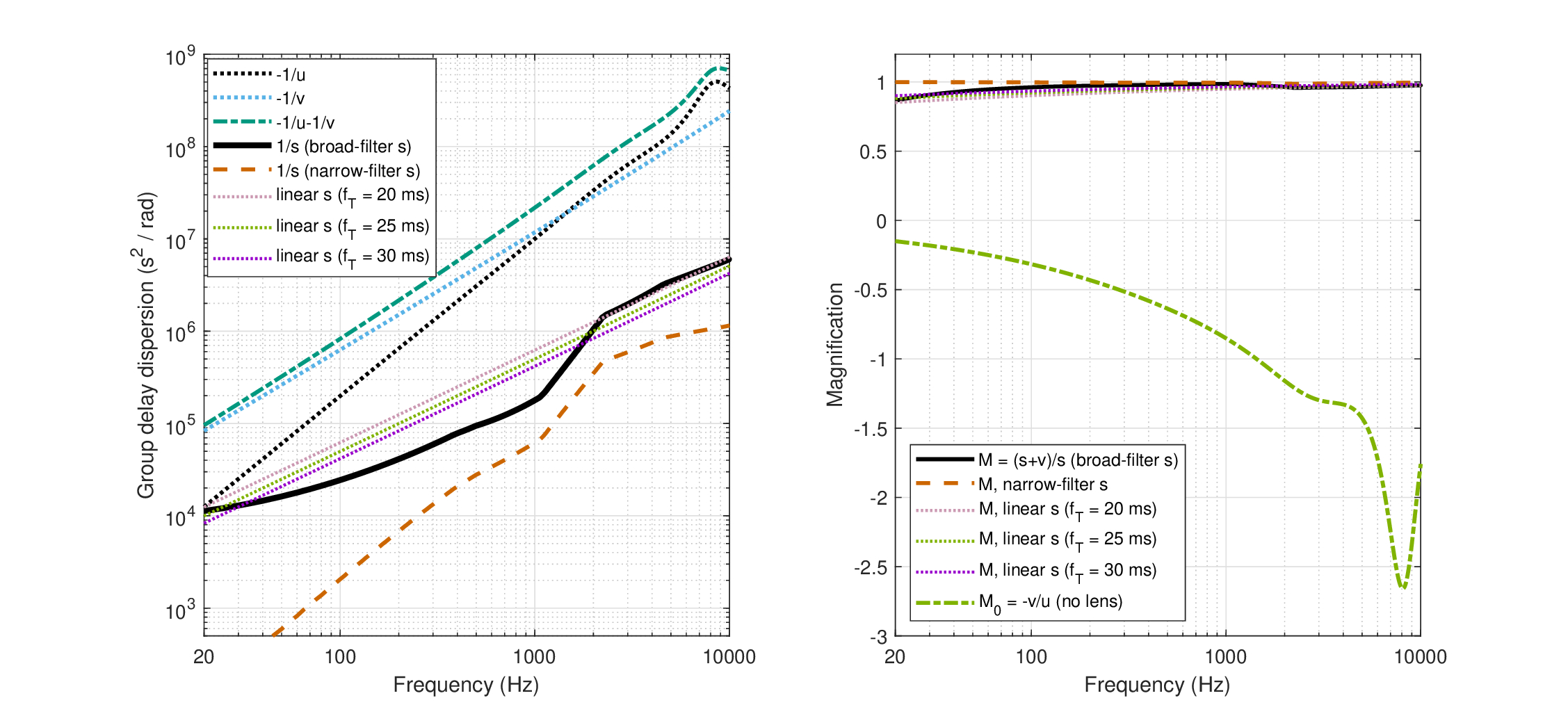
Figure 12.2: Two aspects of the built-in defocus in the human auditory system. Left: Different terms in the temporal dispersive imaging condition, Eq. 12.15. The reciprocal of the negative input dispersion (\(-1/u\)) and negative neural dispersion (\(-1/v\)) are in dotted black and blue lines, respectively. Their sum (dash-dot green) should be compared to the reciprocal of the time-lens curvature(s) (\(1/s\)), which is between one and two order2 of magnitude smaller for the broad-filter large-curvature lens estimate (solid black) and more than two orders of magnitude smaller for the large-curvature narrow-filter estimate (dash red). The intermediate constant focal-time estimates are displayed as well, as the three parallel dotted lines. The differences between the different terms of the equation illustrate how far the system is from sharp focus that would satisfy the imaging condition. Right: The alternative expressions for magnification are displayed. According to \(M = (s+v)/s\), the magnification is relatively flat and asymptotically unity for all the large-curvature cases with the narrow-filter curvature being the closest to 1 (dash red). The other expression for magnification \(M_0 = -v/u\) is unequal to \(M\) when the system is not in focus, but is applicable to lens-less systems. It comes out negative and highly frequency dependent for the parameters we have (dash-dot green). The small-curvature estimates produced curves that were off the chart in all cases and are not displayed here (see text).
It is interesting to consider the effects of \(M_0\), in case it turns out to be the defining magnification constant in the system. First of all, it is negative, which means that it inverts all the images. Second, it also varies considerably throughout the audio spectrum, which implies that similar envelopes that modulate different carriers can be significantly incongruent in duration with respect to one another112, which does not correspond to any known observation about the auditory system at present.
Aside from the fact that the inequality of \(M\) and \(M_0\) underlines the unfocused state of the system, it indirectly affirms the necessity of a lens in the auditory system. The simplest imaging system can be constructed without a lens, only with a pinhole—the pinhole camera. For such a design in temporal imaging, the magnification is exactly \(M_0\) (Kolner, 1997). This suggests that the auditory system must have a lens, even of arbitrary curvature, in order to constrain the magnification and keep it positive. More about this later in the chapter.
Assuming that these results are more or less correct, it is puzzling that the system may be defocused by design for a large range of time-lens curvatures. This question will be tackled directly in §15.5, but we will build towards the answer throughout the subsequent sections.
The defocused nature of the system suggests that it is chirping. There are ample pyschoacoustic data that indeed suggest that the auditory system exhibits natural chirping, which usually shows in asymmetrical sensitivity to up- and down-chirps (e.g., Collins and Cullen Jr, 1978; Nábělek, 1978; Cullen Jr and Collins, 1982; Schouten, 1985; Gordon and Poeppel, 2002). However most of the relevant literature has been concerned either with sinusoidal frequency modulation (FM), or with broadband linear FM (linear chirps), whereas the temporal imaging equations are formulated for narrowband linear FM. A better stimulus paradigm that can be tested against the finding of defocus may be psychoacoustic data based on the Schroeder-phase complex, which emulate linear FM as a periodic signal.
It was briefly mentioned in §10.1 that echolocating animals may use pulse compression signal processing, similar to chirp radars that undo the initial time compression after receiving the reflected pulse. This idea was originally proposed as a model for bat echolocation (Strother, 1961) and was also considered in beluga whales (Johnson, 1992). However, a recurrent problem with this model is that it relies on cochlear dispersion that has to undo the chirp (Altes, 1975). While a large range of delays was measured in different units sampled in the big brown bat's brainstem and inferior colliculus (Haplea et al., 1994), a universal de-chirping of arbitrary calls is unlikely to be found in general, especially given the diversity of call types (Boonman and Schnitzler, 2005). The existence of chirp units in the inferior colliculus is a further evidence that any pulse expansion in bats is partial at best, as they may not have the necessary neural delay lines to produce the matching filters to their returning chirps (Simmons, 1971; Suga and Schlegel, 1973). It is possible that this problem is a manifestation of defocusing of the auditory system in bats, only that it is exploited in different ways in these animals.
12.4 Psychoacoustic glides in temporal imaging
The human auditory dispersion appears to form an imaging system that is out of focus—perhaps by design (Figure 12.2). This entails that for the constant-frequency pulse objects, a chirped image is received and maybe even heard under particular conditions. If this is true, then it may be the underlying cause of psychoacoustic observations that quantify the cochlear phase curvature, only that according to the temporal imaging theory, these observations should be attributed to the entire dispersive system and not only to the cochlea. This interpretation is therefore tested in the remainder of this chapter. Using the temporal imaging equations for defocused images, the human dispersive curvature can be neatly accounted for down to 500 Hz. Frequencies below 500 Hz require a correction that is based on the modulation domain and on irregularities in the cochlear filtering at these frequencies. The most revealing outcome of this exercise, however, is the extraction of what will turn out to be the frequency-dependent aperture time durations. In turn, these values will be shown to closely match direct measurements from the chinchillas, as well as several other measurements done in humans.
12.4.1 Modeling of Schroeder-phase complex curvature measurements
Perhaps the most comprehensive data about the inherent chirping of the human auditory system was measured by Oxenham and Dau (2001a), who obtained estimates for the auditory phase curvature by generating a periodic quasi-linear chirp. This was produced by the broadband Schroeder phase complex at 75 dB SPL (64 dB SPL for each harmonic component; see Figure 12.3), which is thought to approximately cancel out the internal auditory chirp of the system. By adding a pure tone that is one of the harmonics in the Schroeder phase complex, the masking caused by it could be psychoacoustically estimated (Schroeder, 1970; Kohlrausch and Sander, 1995). The curvature estimates were consistent with other measurements and were summarized in Oxenham and Dau (2001a, Figure 8), which is also reproduced in Figure 12.6.

Figure 12.3: Schroeder phase complex with fundamental frequency \(f_0=100\) Hz, \(N=13\), with components between 400 Hz and 1600 Hz (Eqs. 12.28 and 12.29), which is used to mask a 1000 Hz signal with random initial phase. (e.g., Oxenham and Dau, 2001a). Left: With \(C=0\) the masker is highly modulated. Right: With \(C=1\) the masker envelope is nearly flat.
In the Schroeder phase paradigm, a periodically rising or falling glide stimulus is constructed using a sum of \(N\) harmonics of a fundamental frequency \(f_0\),
| \[ p(t) = \sum_{n = n_1}^{n_1+N} \sin(2\pi n f_0 t + \phi_n) \] | (12.28) |
where the phase \( \phi_n\) is given by
| \[ \phi_n = C\frac{\pi n(n-1)}{N} \,\,\,\,\,\, -1 \le C \le 1 \] | (12.29) |
where \(C\) is a curvature parameter and \(n\) is the harmonic number. When \(C=0\) the signal is a normal sine complex tone, but for other \(C\) values, it has a phase curvature that is given by
| \[ \frac{d^2\phi_n}{df^2} = C\frac{2\pi}{Nf_0^2} \,\,\,\,\,\, -1 \le C \le 1 \] | (12.30) |
This formula first appeared in Kohlrausch and Sander (1995) without derivation. The stimulus in the test comprises an additional target stimulus—a pure tone at a frequency that coincides with one of the harmonics (typically \(n=10\)). In Oxenham and Dau (2001a), each target frequency was tested with different \(C\) values in steps of 0.25. The target is minimally masked (lowest threshold) at different \(C\) values that depend on frequency, presumably because this is when the Schroeder complex cancels out the inherent curvature of the auditory system. The net effect is a stimulus that is highly modulated, and thus enables masking release of a sort, by “listening in the dips” between the envelope peaks.
It is instructive to examine the stimuli used in Oxenham and Dau (2001a) in detail. Figures 12.4 and 12.5 show the instantaneous frequencies and envelopes (using the Hilbert transform of Eqs. §6.28, §6.29, and §6.30), respectively, of the seven main stimuli used to obtain Figure 8 in Oxenham and Dau (2001a). Because of the ambiguous nature of the instantaneous frequency concept (see §6.5.3), the linear chirping effect is most visible when the stimulus is bandpass filtered. Therefore, the stimuli are drawn twice—both broadband and bandpass filtered (sixth-order Butterworth), with bandwidth according to the equivalent rectangular bandwidth (ERB) from Glasberg and Moore (1990)
| \[ \mathop{\mathrm{ERB}} = 0.108f + 24.7 \] | (12.31) |
Even after filtering (the auditory filter bandwidth is marked in the figures at \(f_s \pm ERB/2\)) the Schroeder complex is linear only around a narrowband region, whereas outside of it the instantaneous frequency often oscillates rapidly and cannot be meaningfully approximated by a linear slope. A quasi-linear portion is visible in all stimuli but the lowest one, designed to mask 125 Hz pure tones, which has two inflection points within the desired bandwidth. These quasi-linear portions are also visible as being relatively constant in terms of their Hilbert envelopes in Figure 12.5. It can be seen that the 125 and 250 Hz stimuli clearly exhibit spurious periodic chirps within the same ERB that are not the intended downward linear chirp, unless they are bandpass filtered (but note that the curvature is nearly zero for 125 Hz). These ambiguous regions become shorter at higher frequencies, but their effect on the listening tests are unknown.
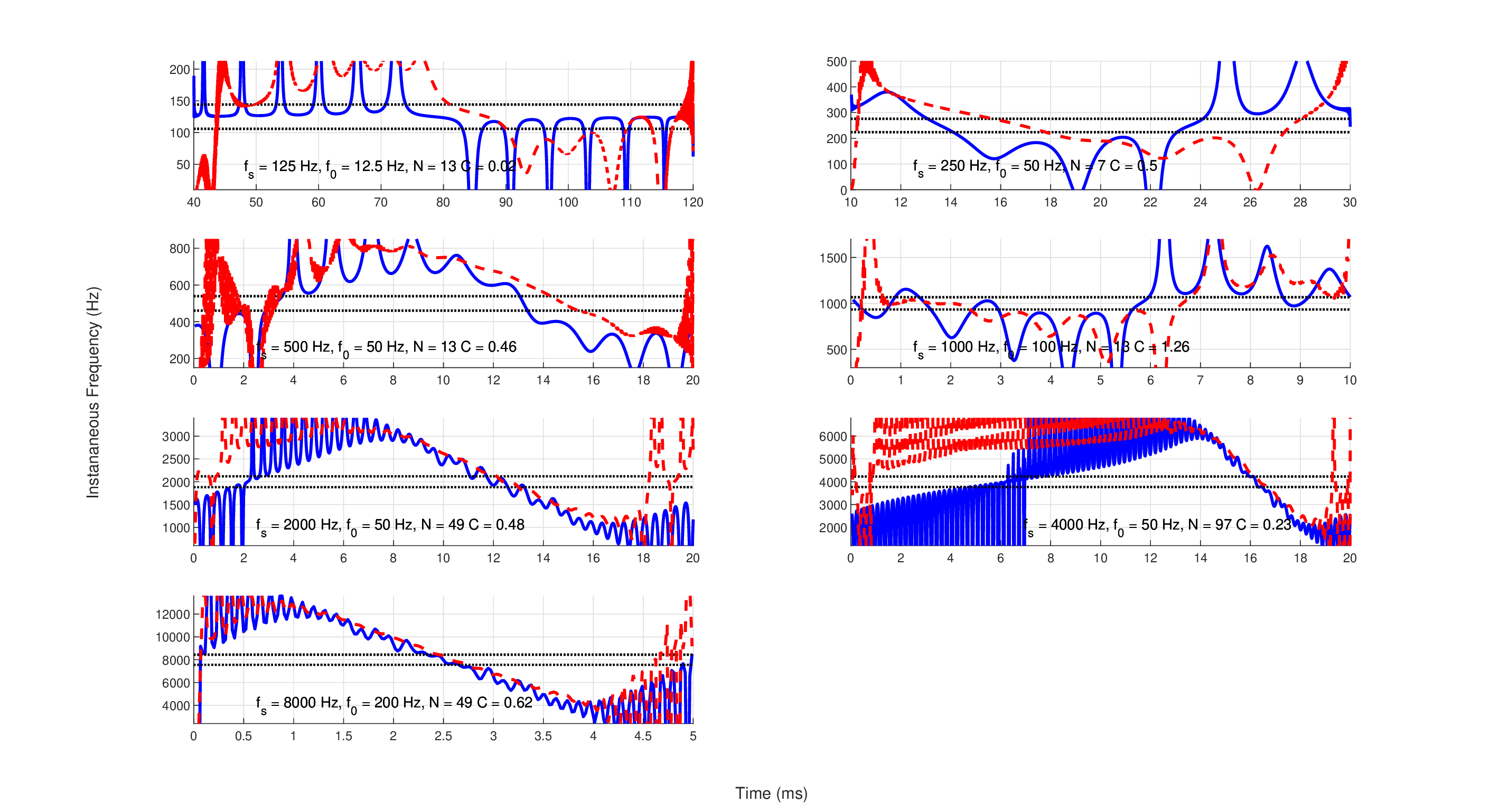
Figure 12.4: The instantaneous frequency of a single period of the seven Schroeder complex stimuli, designed to mask a pure tone frequency \(f_s\) (Oxenham and Dau, 2001a), which elicited the lowest thresholds averaged over four listeners. Each masker contained \(N\) harmonics of fundamental frequency \(f_0\) with curvature value \(C\), as printed on each plot, and computed according to Eq. 12.29. The instantaneous frequencies were computed using the Hilbert transform of the broadband signal (solid blue) and narrowband signal (dash red), which were sixth-order Butterworth bandpass filtered around \(f_s\) (between \(0.6f_s\) and \(1.4f_s\)). In all plots, the limited range of the linear frequency modulation is visible, except for the 125 Hz, where it is smooth but not linear and the curvature is nearly zero. The auditory filter bandwidth around \(f_s\) (one ERB, according to Glasberg and Moore, 1990) is marked with the dotted lines. Note the different time and frequency scales of the different plots.
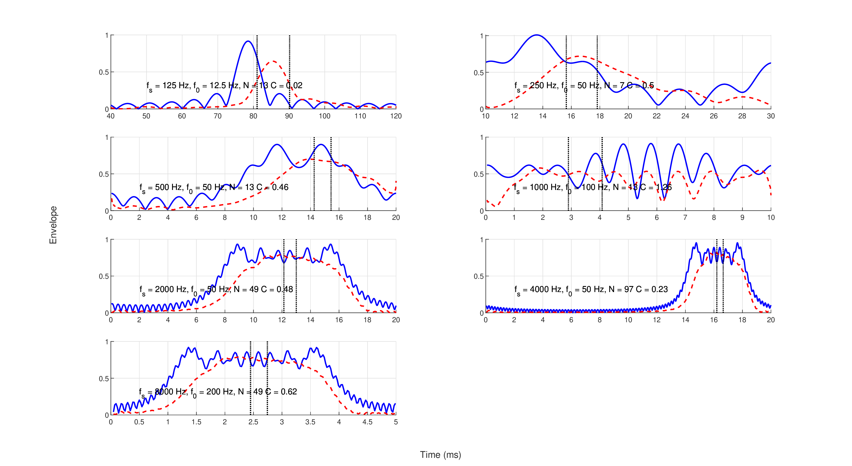
Figure 12.5: The (magnitude) envelopes of a single period of the same seven Schroeder complex stimuli of Figure 12.4. In all cases, the signals had about flat envelope where they were also approximately linearly chirped. Some of the borderline cases in terms of chirping linearity also exhibit fluctuating envelopes. The solid blue curves are broadband envelopes, whereas the red dashed curves are bandpass filtered using the sixth-order Butterworth filters discussed in the text. The dashed vertical lines mark the equivalent duration of crossing one ERB around the signal frequency according to Figure 12.4. Note the different time scales of the different plots.
While Oxenham and Dau (2001a) treated the curvature data as resulting from the cochlear dispersion alone, the temporal imaging theory would require it to be the combination of cochlear, outer-hair cells, and neural dispersive effects. In the simplest case, the imaging condition (Eq. 12.15) is not satisfied, and then the neat scaling expected from imaging (Eq. 12.19) is also not obtained. Instead, using a Gaussian pulse as input, we obtained a closed-form solution that has the same form as the ideal image, but with a complex pulse width (or complex magnification). This was given in Eq. 12.24 and is repeated
| \[ t_1 = M\sqrt{ t_0^2 + 2i\left( u + \frac{vs }{v + s} \right) } \] | (12.32) |
where \(t_1\) is the effective Gaussian pulse width. The additional global phase term in the closed-form solution of Eq. 12.27 is ignored at the moment and will be revisited in §12.6. According to Eq. 12.32, when the imaging condition is not satisfied, the expression in parenthesis does not cancel out, and a real pulse with a linear chirp will result in a complex Gaussian of width \(t_1\). By squaring and inverting the equation,
| \[ \frac{1}{t_1^2} = \frac{1}{M^2} \frac{t_0^2 - 2ix}{t_0^4+4x^2} \] | (12.33) |
with the substitution
| \[ x = u + \frac{vs }{v + s} \] | (12.34) |
It is straightforward to calculate the linear chirp slope \(m_1\) at the output by isolating the imaginary part of this equation, using the Gaussian relations of Eq. §B.21, \(m_1 = -\Im\left(1/t_1^2\right)\)
| \[ m_1 = \frac{2x}{M^2(t_0^4+4x^2)} \] | (12.35) |
This chirp is measured at the output—it is an image that may be perceivable to the listener. Note that we also ignore the effects of neural sampling (§14), as the assumption here is that the chirping information is contained in a single sample—essentially a complete pulse—within the linear duration that sweeps over the pure tone. The stimulus duration, therefore, must be long enough to allow for at least one spike to be fired at the auditory nerve and everywhere downstream.
The complex envelope of the Schroeder complex \(A(0,\omega)\) is locally equivalent to a linear chirp, as its phase curvature is (approximately) constant (Eq. 12.30), with the convenient feature of being periodic. To eliminate the auditory curvature, the Schroeder phase curvature must exactly cancel out the quadratic phase term in the full transform of Eq. 12.23. Therefore, the phase curvature of the input complex envelope \(d^2\angle A(t)/dt^2 = m_0\) undergoes transformation and only then matches \(m_1\), but with an opposite sign. This may be expressed using a complex (AM-FM) pulse (§B.3) with \(t_0^{'2} = t_0^2/(1-im_0t_0^2)\) that has an initial width of \(t_0\). Placing it back in Eq. 12.32,
| \[ t_1 = M\sqrt{ t_0^{'2} + 2ix} = M\sqrt{ \frac{t_0^2}{1-im_0t_0^2} + 2ix} = M\sqrt{ \frac{t_0^2 + i(2xm_0^2t_0^4 + m_0t_0^4 + 2x)}{1+m_0^2t_0^4}} \] | (12.36) |
We impose the condition that the imaginary term under the radical is zero, so to ensure that the image at the output is real and has no chirp. After some manipulation, a quadratic equation is obtained
| \[ m_0^2 + \frac{1}{2x}m_0 + \frac{1}{t_0^4}=0 \,\,\,\,\,\,\,\, x,t_0 \ne 0 \] | (12.37) |
with the roots
| \[ m_0 = - \frac{1}{4x} \pm \frac{1}{2}\sqrt{\frac{1}{4x^2} - \frac{4}{t_0^4}} \] | (12.38) |
and with the constraint
| \[ t_0 \geq 2\sqrt{|x|} \] | (12.39) |
this inequality ensures that \(m_0\) is real (i.e., \(m_0\) and \(t_0\) can be set independently). Otherwise, when \(m_0\) is complex, the output pulse \(t_1\) will anyway contain a chirp that cannot be canceled out.
It appears that determining the precise value of the pulse width \(t_0\) is critical to get a correct estimate of \(m_0\). While the stimulus is continuous, the system can “see” only a fragment of it through a temporal aperture or window, which must not be too short. In the case of equality, \(t_0=2\sqrt{|x|}\), there is only one solution that cancels out the internal dispersion of the system. For larger \(t_0\) values, two perceived curvature minima should have been obtained per subject per condition in the Schroeder's phase experiments. In intermediate cases, when the actual value of \(t_0\) is close to equality, the two curvature minima may merge to a single broad minimum. There is currently no published data to support this effect, although some individual datasets show rather broad and indistinct curvature minima (e.g., Oxenham and Dau, 2001a; Figures 1, 5 and 6 and Shen and Lentz, 2009; Figures 1 and 2). Therefore, we shall start from equality and attempt to minimally perturb the solution from there.
The chirp slope \(m_0\) is defined with respect to the time-dependent phase function, whereas the curvature that appears in Eq. 12.30 was expressed as a frequency derivative. The phase term of the Fourier transform of a linear chirp gives a curvature that is simply \(-1/m_0\)113. Additionally, \(m_0\) was divided by \(4\pi^2\) to convert it to the same units as the frequency curvature in the original paper114.
12.4.2 Initial estimates of the phase curvature and \(t_0\)
The original observations by Oxenham and Dau (2001a, Figure 8) are reproduced in Figure 12.6 (solid curves with black squares and blue triangles) and are used as targets, although their Method 2 was considered more reliable by the authors. The lowest two frequencies measured (125 and 250 Hz) were reportedly less certain than others due to the near-zero curvature involved115, and are also the two that deviate the most from scaling symmetry (dashed black line)116.
The estimate for \(m_0\) that is based on the \(t_0\) model is plotted as well, using the negative-sign solution of Eq. 12.38. The first solution was based on mathematically satisfying the condition of Eq. 12.39 that ensures a real solution using the known system group-delay dispersion parameters, while achieving an optimal fit. This was done by slightly perturbing the equality
| \[ t_0 = 2 \sigma \sqrt{|x|} \,\,\, \mathop{\mathrm{s}} \] | (12.40) |
where the multiplicative factor \(\sigma = 1.058\) was introduced. \(x\) was computed using Eq. 12.34 based on the estimated parameters: the cochlear dispersion \(u\) (§11.5), the broad-filter large-curvature time lens \(s\) (§11.6.3), and the neural dispersion \(v\) (§11.7.3). The obtained \(t_0\) is 6% larger than the theoretical bound. All other large-curvature time-lens models produced nearly identical predictions with \(1.058 \leq \sigma \leq 1.061\), whereas the small-curvature model produced a somewhat poorer fit with a relatively large \(\sigma = 1.19\) (not displayed).
The result is shown as a red dotted line above 500 Hz and dashed gray line below 500 Hz in Figure 12.6. It reveals a close match at frequencies down to 500 Hz, but with poor fits of the 125 and 250 Hz frequencies (continued as gray dashed line and circles in the plot). A much better fit for the two frequencies can be achieved by taking into consideration an external constraint that will be introduced in §12.5.2, which stems from the modulation transfer function analysis of §13.3 and will be discussed in the next subsection. The pulse durations derived from the estimates are summarized in Table 12.1 using the “uncorrected” \(t_0\), which relates to the computation done without the external constraint from the modulation transfer function.
Large individual variations have been reported in curvature estimations (e.g., Oxenham and Dau, 2001a; Shen and Lentz, 2009). For example, under different masker conditions, individual differences in curvature of up to five times were sometimes recorded (Shen and Lentz, 2009; Figure 3), while differences of about two times were common across most conditions (Shen and Lentz, 2009; Figures 3 and 5). Nevertheless, above 500 Hz, the match between the computed \(t_0\) and the data is excellent and only at low frequencies the differences become significant (gray curve in Figure 12.6). Once again, using the large-curvature time-lens values produces a very small change to the values in the table, which are therefore not shown.
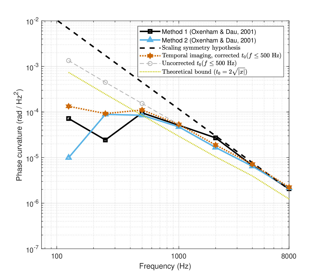
Figure 12.6: The measured and fitted masker frequency slope needed to cancel out the auditory dispersion, based on Schroeder phase complex stimuli (Oxenham and Dau, 2001a). Lines corresponding to Method 1 (solid, black squares) and Method 2 (solid, blue triangles) are reproduced from the data points in Oxenham and Dau (2001a, Figure 8), respectively. The scaling symmetry hypothesis from Oxenham and Dau (2001a, Figure 8) is reproduced as well (dash black). According to the temporal imaging solution (large-curvature time lens), the duration of \(t_0\)—the effective pulse width at the input— is plotted with red asterisks-dot. Theoretically, these values cannot be smaller than the limit in Eq. 12.39, based on the amount of defocus in the system (dot orange). However, at low frequencies (\(\leq\) 500 Hz), the predictions had to be corrected, as a result of the modulation filter bandwidth limitation that will be discussed in §13.4. The uncorrected prediction is marked in dash gray circles.
| Duration (ms) | 125 Hz | 250 Hz | 500 Hz | 1000 Hz | 2000 Hz | 4000 Hz | 8000 Hz |
|---|---|---|---|---|---|---|---|
| Uncorrected \(t_0 \propto \sqrt{|x|}\) | 4.53 | 2.64 | 1.56 | 0.94 | 0.57 | 0.36 | 0.22 |
| Uncorrected \(t_{0,RECT} \propto \sqrt{|x|}\) | 10.67 | 6.21 | 3.67 | 2.21 | 1.34 | 0.86 | 0.52 |
| Corrected \(t_0 \propto \sqrt{|x|}\) | 2.12 | 1.33 | 1.32 | 0.94 | 0.57 | 0.36 | 0.22 |
| Corrected \(t_{0,RECT} \propto \sqrt{|x|}\) | 4.98 | 3.14 | 3.10 | 2.21 | 1.34 | 0.86 | 0.52 |
| \(1/f_s\) | 8.33 | 4.17 | 2 | 1 | 0.5 | 0.25 | 0.125 |
Table 12.1: The different frequency-dependent durations that were fitted to the cochlear curvature data from Oxenham and Dau (2001a). The \(t_0\) durations that are proportional to the internal dispersion \(\sqrt{|x|}\) are given in the first row, and their rectangular equivalent in second row (first row times 2.355). The corrected values that consider the modulation bandwidth at low frequencies are given in the third and fourth rows. The period of the target tone \(1/f_s\) is given in the last row for reference. The three values in italics indicate that they have to be corrected. See text for further details.
12.5 The temporal aperture based on psychoacoustic glide data
12.5.1 The entrance pupil, temporal aperture, and exit pupil
The most striking aspect of the dispersion-dependent fit to the data above 500 Hz is that the pulse width \(t_0\) could be derived independently of the stimulus duration, only as a function of the combined dispersion parameter \(x = u + \frac{sv}{s+v}\), at very close to the minimum theoretical value allowed according to Eq. 12.39. The signal is continuous and much longer than the system is able to process at once. We obtained this signal duration limit \(t_0\), which turned out to be constrained by a function of the internal group-delay dispersions through \(x\) that was estimated independently of the auditory channel response. It can be therefore deduced that \(t_0\) is none other than the temporal aperture of the system—the time-limited window for processing the incoming acoustic signals. More precisely, \(t_0\) is the entrance pupil—the image of the aperture as viewed from the position of the object (see §4.2.2 and Figure §4.5).
While the imaging magnification is smaller than unity (Figure 12.2), there are small differences in the temporal aperture between the object and the image plane, and right at the lens, where the aperture is assumed to be located. At the image plane, the temporal aperture is imaged and appears as the exit pupil. Its duration can be readily computed by using the real part of Eq. 12.33 and Eq. §B.21
| \[ t_1 = M \frac{\sqrt{t_0^4+4x^2}}{t_0} \] | (12.41) |
The same equation may be used to find the actual temporal aperture after the lens, \(T_a\), by setting \(v=0\) and \(M=1\) (see Eq. §B.10, for an example, where the real Gaussian term has the same form, if we set \(x=u\)).
12.5.2 The low-frequency correction
As will turn out in §13.4, using the available values for \(v\) and \(T_a\), as prescribed above, leads to unphysical modulation bandwidths at 125, 250 and 500 Hz for the coherent modulation transfer function117 (Eq. §13.52). In other words, if the 3 dB cutoff frequencies of the low-pass filters that are associated with the modulation transfer functions are calculated using the very same parameter values that are used to obtain the off-fitted 125, 250 and 500 Hz curvatures, then these filters would have modulation bandwidths that are larger than their carriers, which is impossible. Therefore, the current parameter estimates below 500 Hz according to the inequality 12.39 must be wrong. Thus, the cutoff frequencies have to be corrected to only allow modulation bandwidths that are smaller than the carrier. This can be done either by tweaking \(t_0\), \(v\), or both. The effect of \(v\) on the curvature is negligible, whereas reducing \(t_0\) so that the cutoff frequencies at 125–500 Hz are equal to the carrier immediately leads to a much better fit of the off 125 and 250 Hz curvature points, and a little improvement to the off 500 Hz point. In order to obtain the corrected values for \(t_0\), the new aperture was used in Eq. §13.52
| \[ T_a = \frac{ 4\sqrt{2}|v| }{\mathop{\mathrm{FWHM}}} 0.9\omega_c \] | (12.42) |
where 0.9 is the arbitrary fraction of the carrier \(\omega_c\) bandwidth that replaces the previous bandwidth118. We are interested in non-rectangular (Gaussian) aperture duration, which is why the expression is divided by \(\mathop{\mathrm{FWHM}} \approx 2.355\)119. Finally, the new aperture duration of Eq. 12.42 has to be back-propagated to the entrance of the system, to obtain the entrance pupil \(t_0\). This is done with
| \[ t_0 = \sqrt{\frac{T_a^2 \pm \sqrt{T_a^4 - 16u^2}}{2}} \] | (12.43) |
This expression was derived from Eq. §B.10 by comparing the real Gaussian width to \(T_a\) and solving the biquadratic equation in \(t_0\). Note that with the corrected values of the dispersion term \(x\), \(m_0\) has to be complex to satisfy Eq. 12.37, which means that there will be a glide at the output anyway—potentially an audible one. Therefore, \(x\) must be corrected as well to satisfy the inequality 12.39. It was done by using the new \(t_0\) from Eq. 12.43 with the empirically obtained inequality 12.40. However, both solutions in Eq. 12.43 are complex, so we shall discard the imaginary part of the obtained \(t_0\) and note that this solution is provisional.
Results for the three tweaked points are displayed in Figure 12.6 (dotted red curve). In addition to the corrected \(t_0\), the corresponding \(x\) values were reiterated using Eq. 12.40 to force zero chirping at the output—something that made the fit a little worse. The required changes in \(x\) are significant, but there are no other data to guide this correction and pinpoint which parameter(s) within \(x\) should be specifically modified (i.e., \(u\), \(v\), or \(s\)).
The final entrance and exit pupil and the aperture time values are summarized in Table 12.2. As can be seen from the table, the differences between the three measures tend to be small, but are more pronounced at low frequencies. Note that the term temporal aperture is used to to refer to the device or feature that imposes the temporal constriction in the signal path, whereas aperture time is the particular duration that is associated with it.
| Duration (ms) | 125 Hz | 250 Hz | 500 Hz | 1000 Hz | 2000 Hz | 4000 Hz | 8000 Hz |
|---|---|---|---|---|---|---|---|
| \(t_0\) (entrance pupil) | 4.98\(^*\) | 3.14\(^*\) | 3.01\(^*\) | 2.15 | 1.28 | 0.79 | 0.44 |
| \(T_a\) (temporal aperture) | 9.13\(^*\) | 4.87\(^*\) | 3.31\(^*\) | 2.21 | 1.30 | 0.80 | 0.44 |
| \(t_1\) (exit pupil) | 5.27\(^*\) | 3.35\(^*\) | 3.33\(^*\) | 2.32 | 1.35 | 0.83 | 0.47 |
| \(\Delta t_{opt}\) | 3.18 | 1.96 | 1.19 | 0.72 | 0.43 | 0.26 | 0.13 |
| \(T_a/\Delta t_{opt}\) | 2.87 | 2.49 | 2.78 | 3.09 | 3.07 | 3.08 | 3.40 |
Table 12.2: The entrance and exit pupils and aperture times of the full auditory system, based on Eqs. 12.40 and 12.41. The entrance pupils are the corrected \(t_{0,RECT}\) values from Table 12.1, where for the 125, 250, and 500 Hz values (marked by an asterisk) were corrected using modulation filter considerations (see text). The \(T_a\) values were computed by setting \(x=u\) in Eq. 12.41 (the effect of \(s\) is multiplicative chirping and thus does not matter here). The exit pupil values were calculated using Eq. 12.41. Additionally, the theoretical values that exactly balance the geometrical and dispersive blurs are given with \(\Delta t_{opt}\), which was computed using Eq. §13.21. The ratio between the actual aperture stop and the optimal values are given in the last row, showing that geometrical blur is three times larger than dispersive blur, on average. All values are equivalent rectangular bandwidths in milliseconds.
Several causes may account for the anomalous low-frequency results. As was discussed when \(u\), \(s\), and \(v\) were initially estimated, there are some uncertainties associated with all of them, which can be substantial at low frequencies, where they were sometimes extrapolated. Another possible cause for the discrepancy in \(x\) is that even the allowed modulation bandwidth results in over-modulation, since the narrowband approximation breaks down and the governing equations no longer hold, as higher-order dispersion terms become dominant (Bennett and Kolner, 2000a).
Another likely cause for the anomalous behavior we observed below 500 Hz and the unusually broadband channels is that the cochlear filters are not truly bandpass toward the apex, but rather low-pass. This has been observed in several studies in the last years that specifically targeted the apical cochlear mechanics, using various novel imaging techniques that do not damage the delicate cochlear structures, where noticeable differences have been observed in comparison with the better studied basal mechanics. For example, the guinea pig apex (characteristic frequencies, CF \(<\) 2 kHz) was tested in vivo, where it was found that the cochlear response is low-pass, while only neural filtering imposed the bandpass response (Recio-Spinoso and Oghalai, 2017). Using the scaling property of the cochlea to transform this frequency range from the guinea pig to humans, it maps to CFs below about 900 Hz (Greenwood, 1990; Figures 1 and 4). The physical modulation limitation that resulted in the above correction holds below 660 Hz, according to Figure §13.2. If a similar response characterizes the low frequencies in humans as in the guinea pig, then its effect is to change the aperture duration and shape, and possibly tamper with the neural dispersion computation. In any event, a low-pass component in the dispersive system would challenge the narrowband approximation and may have to be replaced with a more accurate model. The guinea-pig findings are compounded by a followup study that additionally found that, unlike the group delay in basal locations, in apical locations the group delay is almost independent of level (Recio-Spinoso and Oghalai, 2018). Another study of the guinea-pig found little to no variation in best frequencies between apical and middle cochlear sites (different from basal sites), which also exhibited very little group delay dispersion in comparison with the standard place-model predictions (Burwood et al., 2022). It was also demonstrated that the outer hair cells are responsible for distributing the mechanical response between apical sites and among auditory nerve channels. Low-pass responses were also shown in the gerbil, where CFs in the apical first turn also exhibited a different compressive nonlinearity than either the second or the third (basal) turns (Dong et al., 2018). Finally, Warren et al. (2016) found that the displacement amplitude of the basilar membrane in the apical turn of the guinea-pig was considerably smaller than in more basal sites, and that the motion was significantly larger on the reticular lamina—that is, after the outer hair cell bodies. It was suggested that these differences are fundamental, so much so that straightforward scaling of the cochlear properties from basal data to apical sites may be invalid (Dong et al., 2018).
In humans, in a study that compared stimulus-frequency and distortion otoacoustic emissions (OAEs), it was found that OAE recordings returning from the cochlea have three regions that are separated by two bends in their phase response: basal above 2500 Hz and apical below 900 Hz (Christensen et al., 2020). This matches the remapped frequency range estimate from the guinea pig data by Recio-Spinoso and Oghalai (2017) above.
12.5.3 Comparison with temporal windows from psychoacoustic literature
The entrance pupil values we computed, which refer directly to the duration of the input stimulus, can now be compared with some psychoacoustic data from the literature.
Values of \(t_0\) may be tested against independent psychoacoustic data measured by van Schijndel et al. (1999) of intensity discrimination tests of Gabor pulses of different durations (“shape factors”), but equal power. The masking thresholds of three subjects were measured at various levels using a pink-noise masker. Similar to Gabor's logons (Gabor, 1946), the authors hypothesized that the auditory stimuli may be perceived in multiple time-frequency grid windows, but that with the right choice of time-bandwidth product the number of active windows can be minimized. For a Gaussian envelope \(\exp\left[-\pi (\alpha f_c t)^2\right]\), the shape factor \(\alpha\) produced the worst just-noticeable intensity difference for \(\alpha = 0.3\) with carrier \(f_c = 1000\) Hz and \(\alpha = 0.15\) with \(f_c = 4000\) kHz carrier (van Schijndel et al., 1999; Figure 3). By equating these coefficients to the standard Gaussian used throughout this chapter (Eq. 12.21), which explicitly contains the entrance pupil, we obtain \(t_{0,RECT} = \mathop{\mathrm{FWHM}} /(\sqrt{2\pi} \alpha f_c)\), which results in 1.6 ms at 4 kHz and 3.1 ms at 1 kHz. These values are longer than the values obtained in the present study of 0.8 ms at 4 kHz and 2.2 ms at 1 kHz (see Table 12.2). The data points are shown alongside the temporal aperture and entrance pupil values from the present study in Figure 12.7.
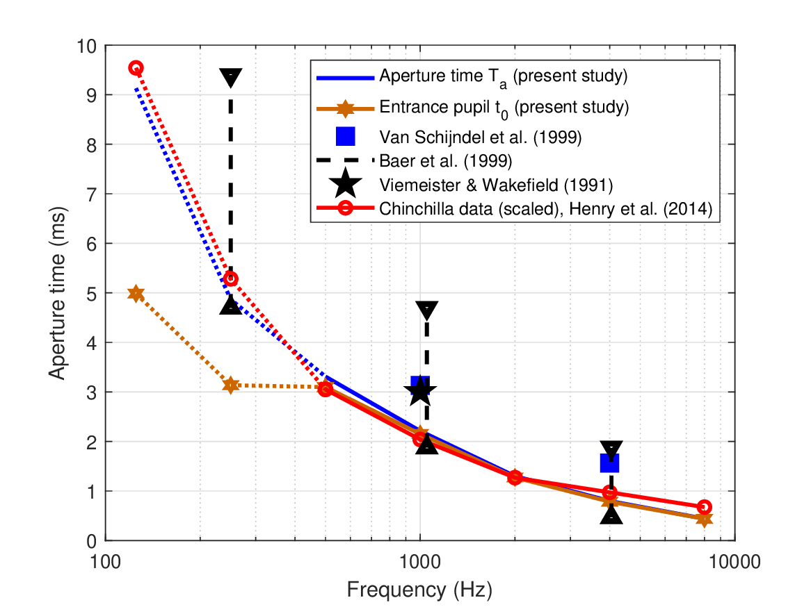
Figure 12.7: The aperture time and entrance pupil estimates from the present study (second and first rows in Table 12.2, respectively) and comparable estimates from literature. All values are given in equivalent rectangular durations. Psychoacoustic data are taken from van Schijndel et al. (1999), Baer et al. (1999) and Viemeister and Wakefield (1991). The physiological data from (Henry et al., 2014b) were scaled for the slight difference in the cochlear mapping between the chinchilla and human (Greenwood, 1990). The present data are uncertain at 125, 250, and 500 Hz because of the exact relationship between the carrier and modulation bandwidths (see text), but they provide a reasonable fit to the curvature data from Oxenham and Dau (2001a). Data for these frequencies from Henry et al. (2014b) were linearly extrapolated from the reported 500–8000 Hz data.
The van Schijndel et al. (1999) experiment was replicated with three other subjects and extended to 250 Hz and additional conditions by Baer et al. (1999), whose results were added to Figure 12.7. The mean results for 1 and 4 kHz of van Schijndel et al. (1999) were replicated, but higher individual variability of the pulse was observed in different intensity conditions. The test included a quiet condition that in absolute level was closest to 40 dB SPL (Baer et al., 1999; Figure 2), as was used to derive our temporal aperture. At 1 kHz, the peaks are distributed between 1.9 and 4.7 ms—longer in the quiet condition, and shorter but less peaky at the 40 dB masked condition. Similar ranges were obtained for the other frequencies, which always contain the estimates from our theoretical prediction, as can be seen in Figure 12.7 (dash lines, triangles).
The value we obtained of \(t_{0,RECT}\) at 1 kHz (2.2 ms) is also smaller than the equivalent rectangular width of a single “look” of the order of 3 ms at 1 kHz, as was estimated in Viemeister and Wakefield (1991)120.
The discrepancy between the values may be attributed to individual variations, possible level-dependent differences in all the various studies, and essentially different methods that may not exactly tap into the same quantity.
12.5.4 Comparison with physiological chinchilla data
A much more precise comparison to our aperture time can be made using physiological data of the temporal windows of anesthetized chinchillas from Henry et al. (2014b). The data are based on single-unit measurements of auditory nerve fibers, whose response to Gaussian white noise input was used to derive the second-order Wiener kernel of the system. The temporal windows of normal-hearing controls (10 animals, 143 fibers) were obtained at different frequencies by computing the first eigenvector of the second-order Wiener kernel and applying Hilbert transform on it. The Hilbert envelope facilitated a direct estimate of the temporal window and it was calculated at different levels relatively to the peak. Since the relative cochlear frequency maps of humans and chinchillas are almost identical (Greenwood, 1990), it is possible to directly compare the human and chinchilla data with minimal error. Nonetheless, a scaling correction was applied by using the chinchilla's cochlear map to derive the relative cochlear place for the reported data, and then obtain the equivalent place-frequency for the human cochlea (Greenwood, 1990). From these values, slightly modified temporal window estimates were interpolated from the 50% (FWHM) temporal window values from Henry et al. (2014b, Figure 7, top) for characteristic frequencies of 500–8000 Hz, which are reproduced in Figure 12.7. Once converted to equivalent rectangular widths, these values are directly comparable to the aperture time values of the second row in Table 12.2.
The linear regression trend line from Henry et al. (2014b, Figure 7, top) was linearly extrapolated to have estimates also for 125 Hz—9.54 ms and 250 Hz—5.28 ms. Note that the two extrapolated values are expected to be a little longer, because the chinchilla's frequency map deviates from the power law below 500 Hz (Greenwood, 1990). The differences between the present aperture time estimates and the transformed chinchilla's values are 4.3–8.4% for frequencies below 2000 Hz, but at 4 kHz it is 18% and at 8 kHz it is 34.6%. This gives an average error of 12% for the seven frequencies. Regardless, these aperture time estimates are in excellent agreement with the present study, given the wildly different methods and conditions used to obtain them, as well as the uncertainty in the dispersion parameters and the possible low-frequency anomaly.
It is remarkable that the Gaussian pupil shape gave such close results to the physiological data of the chinchilla. In addition to the specific temporal window values, the Henry et al's paper provided one instance of an actual window function that was estimated using the Wiener kernel method (Henry et al., 2014b; Figure 1E). Using a zero crossing estimate from the figure, the carrier is about 3.9 kHz, for which the authors provided a 50% temporal window duration of 0.93 ms. The envelope is replotted in Figure 12.8, after centering and normalizing the peak. The window has a long tail, which extends for another 2–3 ms after the peak. Using the duration from the paper and the present estimate of the temporal aperture at 3.9 kHz (0.87 ms), it is possible to compare the measurements to a theoretical Gaussian pupil. Gaussian pupils of these two durations are plotted in Figure 12.8 as well. Excluding the tail, the measured and theoretical pupils are nearly identical. This suggests that the Gaussian pupil function may be a valid approximation for the aperture for most of the stimulus121. However, the Gaussian pupil may not account for slow and low-energy signal decay and possible aberrations induced by the asymmetrical tail (§15.9).
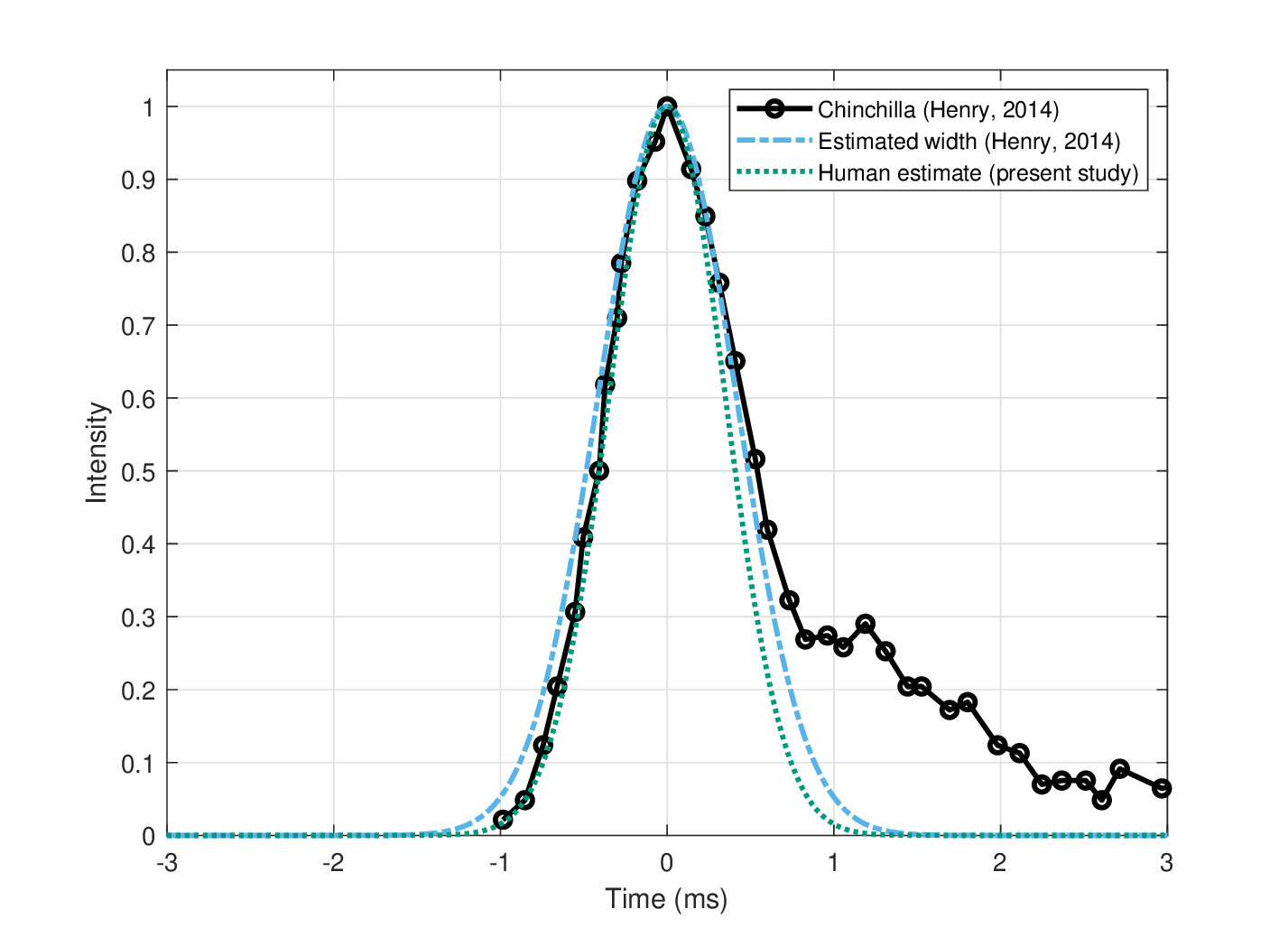
Figure 12.8: An example of a temporal window of the chinchilla measured at about 3.9 kHz (black solid circles), obtained from data by Henry et al. (2014b, Figure 1E). The authors provided the 50% window duration, which is used in a Gaussian pupil function (blue dash-dot line). The present-study estimate from human data for the same frequency has a slightly narrower duration, which is plotted as another Gaussian pupil in green dotted line.
12.5.5 Comparison with psychoacoustic beating data
As a final test of the temporal aperture values and shape, we can compare the present values to psychoacoustic results from literature that quantify the beating threshold between two tones. Acoustic interference has been localized to be taking place within the auditory filter and the periphery and anyway not centrally (Krumbholz and Wiegrebe, 1998). In §8.2.9, we derived an expression for the frequency range of beating between two tones with frequency difference \(\Delta f\), based on nonstationary coherence theory, which depends only on the temporal integration time of the hypothetical intensity detector with a Gaussian window. The FWHM of the detector was set as a frequency spacing criterion, as beating can be distinctly observed only for \(\Delta f < 0.44/T\). It is interesting to examine how the temporal aperture compares with published estimates for this threshold, by setting \(T=T_a\). Results from literature are compiled from Plomp (1964a), Plomp and Mimpen (1968) and Plomp and Steeneken (1968), and to a rule of thumb provided by Moore (2002), which sets the limit of beating at maximum spacing of \(\Delta f \approx 1.25 \mathop{\mathrm{ERB}}\)122. The results are all plotted in Figure 12.9. As the curves show, all frequencies but 250 and 500 Hz are within the spread of the data from literature. This discrepancy reinforces the suspicion that the low-frequency data may be misestimated. Nevertheless, the beating measurement may provide an alternative and more direct way to estimate \(T_a\) that is independent of all other dispersion parameters. Thus, if we use Moore's \(1.25\mathop{\mathrm{ERB}}\) law as approximating the literature average, we would obtain \(T_a=6.8\) ms at 250 Hz and \(T_a = 4.5\) ms at 500 Hz. These values are significantly longer (by 29% and 26%, respectively) than the values from Table 12.2. The value found at 1 kHz is also longer (17%) than the dispersion-derived value. All other beating duration are less than 11% different from the estimates, and the seven frequency average difference is 14%.
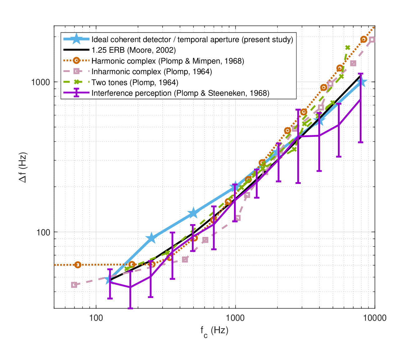
Figure 12.9: Auditory beating perception of two tones expressed through their frequency spacing \(\Delta f\), as a function of average frequency \(f_c\). Predictions according to Eq. §8.81 and the aperture time values from Table 12.2, row 2, are plotted in solid blue stars. Different data from literature are plotted in comparison, which are based either on harmonic complexes (Plomp, 1964a; Plomp and Mimpen, 1968), inharmonic complexes (Plomp, 1964a), or two-tone interference (Plomp, 1964a; Plomp and Steeneken, 1968). The additional rule of thumb of \(\Delta f \approx 1.25 \mathop{\mathrm{ERB}}\) by Moore (2002) is plotted for reference too.
12.6 The global quadratic phase term
The role of a finite aperture is critical in suppressing the oscillations of the global quadratic phase term that appears in the imaging transforms (e.g., Eqs. 12.19, 12.22, and §13.20) and has been neglected earlier. The inclusion of the global phase term is of no consequence in intensity images (because of squaring), but can severely distort the amplitude image if it is not truncated by the aperture.
The quadratic phase functions at the seven frequencies are shown in Figure 12.10 along with where the (rectangular equivalent) exit pupil (i.e., the image of the aperture) truncates them. In the case of the large-curvature time lens (all models), there is no effect of the quadratic phase within the limits of the exit pupil, as the amplitude hardly drops from its maximum value. Therefore, the quadratic phase is effectively constant within the temporal window and no plausible risk of distortion is present (solid black curves in Figure 12.10). In contrast, the small-curvature time-lens exhibits half a cycle of the quadratic phase within the limits of the exit aperture. While it does not oscillate within the aperture, the effect of such a lens may still be distorting. It might also cause a loss of perceived loudness, as there is a smaller amount of power per image in comparison to the large-curvature image.
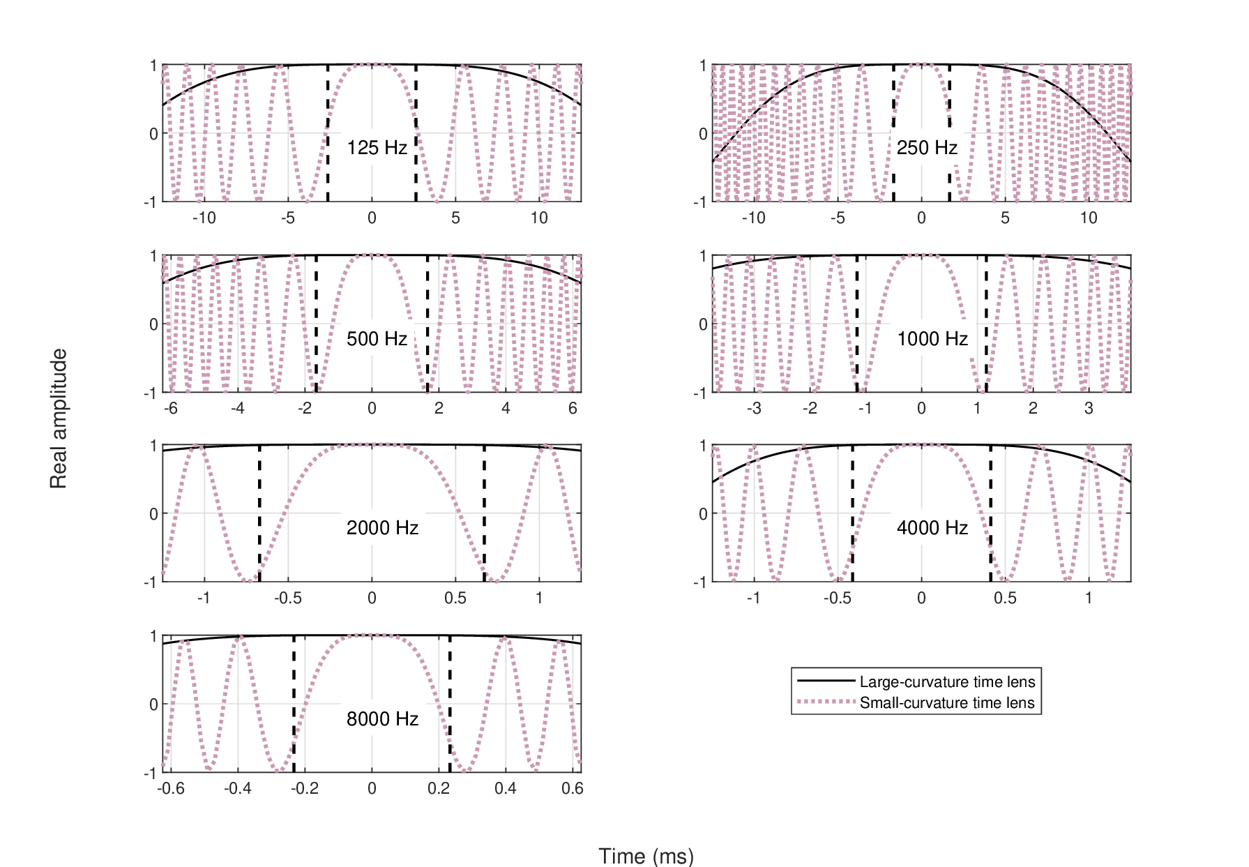
Figure 12.10: The global quadratic phase term in the imaging transform, \(\exp\left[\frac{i\tau^2}{4(v+s)} \right]\), at the seven frequencies tested above. This phase does not matter in intensity imaging, but may distort the image in amplitude imaging if left un-windowed. Therefore, it is important that the temporal aperture truncates the quadratic phase function while it is still in the main lobe, where the amplitude magnitude is as close to 1 as possible. With the small-curvature time lens (red dot), it is never the case, as the phase completes up to half a cycle within the window, as can be seen by the vertical dashed lines that mark the (rectangular) \(\pm t_1\) times, obtained from Table 12.2. If we use the large-curvature time-lens data (solid black), then the problem disappears completely, as the phase becomes effectively constant within the aperture time. Only the real part of the complex envelope amplitude is displayed.
For additional validation in the context of the Schroeder-phase complex data, the system including the phase term can be analyzed in closed form. Starting from the full solution of Eq. 12.23
| \[ a_n(\zeta _2 ,\tau ) = a_0 t_0 \sqrt{ \frac{\frac{s}{v + s}}{2 \left[ \frac{t_0^2}{2} + i\left( {u + \frac{{vs }}{{v + s}}} \right) \right]}} \exp \left[ {\frac{{i\tau ^2 }}{{4(v + s)}}} \right] \exp \left\{ \frac{-\left(\frac{s}{{v + s}}\tau\right)^2}{ 4\left[ \frac{t_0^2}{2} + i\left( {u + \frac{{vs }}{{v + s}}} \right) \right]} \right\} \] | (12.44) |
According to the formalism of §B.3, the frequency slope of the first quadratic phase term is \(m_g = \frac{1}{2(v+s)}\). Using the complex output pulse solution of Eq. 12.36, the frequency slopes of the two quadratic phase terms in Eq. 12.44 can be summed, according to Eq. §B.15. Using \(m_g\), then once again the imaginary part of the output signal should cancel out when applying an external chirp with slope \(m_0\). This can be written as
| \[ m_g + \frac{m_0t_0^4 + 2m_0^2t_0^4x +2x}{M^2\left[t_0^4(1+2xm_0)^2 + 4x^2\right]} = 0 \] | (12.45) |
which translates into this quadratic equation
| \[ 2t_0^4x(2m_g xM^2+1)m_0^2 + t_0^4(1+4x m_g M^2)m_0 + 2x+ m_g M^2(t_0^4+4x^2) = 0 \] | (12.46) |
Given the values obtained of \(t_0\), \(x\), and \(M\), all the terms involving \(m_g\) are negligible in comparison with the terms that do not contain it, which asymptotically reduces this quadratic equation to the original one in Eq. 12.37. Therefore, this configuration is indistinguishable from the full system, at least as far as the psychoacoustic phase curvature is concerned.
The importance of amplitude imaging at this stage is not entirely well-understood. In the case of intensity imaging, the entire transformation is squared, so that the quadratic phase is anyway canceled out.
12.7 Discussion
We presented the derivation of the basic temporal imaging theory according to Kolner and Nazarathy (1989) and Kolner (1994a) and applied it to the auditory system of humans. The system appears to be out of focus by design, which can be used to account for its chirping property (glides). Several important observations could be made based on the successful modeling of the psychoacoustic curvature data based on the theory. Most central to them is the identification and estimation of the temporal aperture.
12.7.1 The imaging equations
The basic equations of the temporal imaging theory were adopted from Kolner (1994a), almost verbatim, only with occasional changes in notation. The temporal imaging equations are exactly analogous to those of Fourier optics (Goodman, 2017), as long as we exchange the spatial modulation for temporal modulation, and with two less spatial dimensions. Temporal imaging is conceptually more complex because it overloads the time domain with both modulation and carrier evolution, whereas in light frequencies of spatial optics the two are distributed in different dimensions and domains that have close to no interaction. This mixture between the carrier and modulation domains is propagated inside the hearing system, as the two frequency ranges largely overlap, sometimes within the same pathways.
12.7.2 Inherent auditory defocus
Unlike Kolner's applications and most others' in the burgeoning field of ultrashort pulse imaging, we were led to concentrate on a defocused system configuration that appears to be relevant to the human auditory system, and thus has a very different parameter space than is typical in optics. Many attempts were made by the author to perturb the obtained system parameters (not presented here, except for two time-lens curvature data sets) using alternative datasets from literature that may be used for dispersive parameter derivation, but all led to the inevitable conclusion that the defocus term is too large to be an estimation error (see Figure 12.2). It begs the question: Why is the auditory system configured to be defocused? In optical imaging systems, defocusing is sometimes used to achieve selective sharp focusing on one object, while blurring undesirable parts of the scene. We will tie this principle of operation to coherence over the next chapters and specifically in §15.5.
Perception of the auditory phase curvature was hitherto associated with the cochlear dispersion alone, but was modeled here successfully using a single pulse image, whose imaginary part that normally produces a linear chirp was set to zero. The internal chirp that had to be canceled out can be understood as a defocusing side-effect (formally, an aberration)—which we represented by \(x\)—the defocusing parameter. It may be taken as an additional confirmation that the auditory system is inherently defocused.
It is possible to obtain another bit of intuition about the defocus, by computing how the auditory system balances with geometrical and diffraction blur (see §4.2.2). In good optical designs, the two can be traded off to optimize the image sharpness, so that the defocus is minimal, but also not much object detail is lost to diffraction, so a diffraction-limited image can be realized. We will obtain the formulas to compute this optimum in §13.2.2, but the results according to Eq. §13.21 are given in the bottom two rows of Table 12.2. As can be seen, the computed durations of the auditory temporal aperture are suboptimal, in that they are about 2.4–3.5 times longer than the optimum. This means that the auditory system works above its dispersion limit, within its geometrical range. In other words, the images are not significantly corrupted by dispersive effects, which would have required much shorter aperture times to be distinctly noticeable. Thus, the auditory system is not dispersion-limited, unlike the eye that is close to being diffraction-limited, at least for average pupil sizes (§4.3).
12.7.3 The temporal aperture
The temporal aperture is a mandatory component in any system that dynamically processes signals over time and is inevitable in any imaging system of finite extent. However, the temporal aperture mathematics does not indicate where it is exactly localized in the auditory system. Various psychoacoustic models have attempted to approximate the temporal response of the auditory system, (see §E.1 for a short review), but the temporal imaging theory may only agree with something like the multiple-look model (Viemeister and Wakefield, 1991) or variations thereof, which assume a discretized representation of sound without committing to a specific physiology. Our aperture analysis became better grounded with the ability to closely match the obtained psychoacoustic results to direct physiological measurements of the temporal window of the chinchilla by Henry et al. (2014b). This surprising finding serves two important purposes. First, it localizes the aperture in the cochlea and auditory nerve—probably behind (after) the time lens. The neural firing itself is the most natural candidate to constitute the aperture, given its finite sampling period. However, at low frequencies, where the cochlear mechanics appears to behave differently, there may be a temporal effect on the aperture of the specific mechanical filtering as well. Second, it provides a very strong indication that the Gaussian function can well describe the aperture shape, at least around its center. This will be of utmost importance in the chapters dealing with modulation transfer functions.
Another surprising fact is that the apparent general validity of the inequality 12.40, from which we derived the temporal aperture. This expression was motivated through the particular problem of accounting for the stimuli in Schroeder phase complex experiments and it appeared as a mathematical-physical constraint to the actual solution. It is likely that this inequality can be motivated and derived in a more general way that is independent of this particular problem. Once such an approach is found, it may become easier to develop further insight about temporal imaging in the auditory system, and in defocused systems in particular.
12.7.4 The auditory dispersion parameters
The convergence of the numerical values obtained by wildly different methods is an important indicator that applying the temporal imaging theory to the auditory system is warranted. The temporal aperture function constitutes the final parameter that is needed to describe the basic imaging system of hearing, along with \(u\), \(v\), and \(s\). Interestingly, we saw how the temporal aperture duration above 500 Hz can be very closely approximated by a combination of the other three parameters, which serve as a mathematical lower bound that enabled the cancellation of the internal chirp (Eq. 12.39). The bound called for a factor of 2, whereas we obtained 2.116 as a preferred factor to optimize the fit to the data (\(\sigma = 1.058\) in 12.40). It is likely that a more precise estimate of the other parameters will lead to it being even closer to 2. This will also ensure a unitary minimum for the curvature masking of the Schroeder phase complex, per frequency band.
There was much uncertainty with respect to values that time-lens curvature should take, according to the different auditory filter models §11.6.3. While all the models produced a very close fit to experiment with the right \(\sigma\), the broad-filter time lens curvature minimized it, while achieving a somewhat closer fit. In a later analysis we shall explore the possibility that the system can accommodate the time-lens curvature, somewhat similarly to vision (§16.4.2).
Throughout this analysis, we have excluded one key component from the system. To account for the continuous nature of the signal, the aperture has to be triggered at a certain rate. In the moving image camera it is achieved with a shutter (e.g., a rotary disc shutter in analog cameras). The solution provided above was derived based on a single sample, so the shutter function was implicit. If the auditory nerve firing represents the temporal aperture and the sample, then the neural spiking rate may be thought of as a (nonuniform) trigger that works as a shutter. This will be explored in more depth in §14.
12.7.5 Pinhole camera design
The auditory imaging system appears to combine a short temporal aperture and a time lens with uncertain, and possibly variable, curvature. This architecture closely resembles the pinhole camera design. As the time-lens curvature was based on relatively few data points and its effect on the perceptual data appears to be limited (because of its small curvature), its role and very existence remain somewhat uncertain at this stage of the analysis. If the lens would be altogether missing—in line with standard cochlear models that do not attribute any phase-modulatory role to the organ of Corti / outer hair cells—then the system would assume the “classic” temporal pinhole camera design (Kolner, 1997). In the pinhole camera, the magnification depends on the input and neural dispersion alone (\(M=-v/u\), Kolner, 1997), which would yield an inverted (time-reversed) image, as both \(u\) and \(v\) are negative, according to our analysis. In contrast, the scaling involved in the full system with time lens depends on the other expression of the magnification \(M = v/(s+v)\), which is positive and close to unity (see Figure 12.2, right). Keeping the image non-inverted may be one significant role of the time lens. A counter argument, then, may be that such time-reversal has not been documented in the auditory literature because it can only be detected on a very short time scale in narrowband. However, the values of the \(-v/u\) magnification are also extremely variable in frequency, which does not seem like a desirable design characteristic for the auditory system.
Despite its unlikeliness, one of the most important features of the pinhole camera is that it has a theoretical infinite depth of field. This also implies an atypically large depth of focus. Similar properties can be expected from the single-lens system with very small aperture. This aspect of the system will be explored in §15.
12.7.6 Absorption and high-order dispersive aberrations
In the entire analysis, there was no obvious need to invoke the group-delay absorption (imaginary parts of the \(u\), \(v\), and \(s\) parameters) to model the data with a reasonably convincing fit and, indeed, such attempts have not been presented. It may provide limited confirmation for the validity of neglecting the absorption in the dispersion equation (§10), at least at high frequencies. Thus, the auditory system may form images in a dispersion-dominant fashion, just like the original temporal imaging theory by Kolner and Nazarathy (1989). Nevertheless, in modeling the perceptual curvature response there were some uncertainties involved at low frequencies, which may be accounted for by high-order dispersive aberrations or by absorption, as well as by an altogether different filter topology (e.g., low-pass instead of bandpass). Theoretically, the effects of such an absorption could be image deformation and chirping that are unaccounted for by the input chirp \(m_0\) or the simple defocus term \(x\). Except for possible over-modulation at low frequency carriers, there is no data to support these claims at present.
The need to elucidate the significance of absorption receives more currency in §F, where the entire dispersive parameter set (\(u\), \(v\), \(s\), and \(T_a\)) is re-derived using strictly psychoacoustic effects and available data, including the phase curvature and beating effects explored earlier. This alternative solution is largely consistent with other results in this work based on our earlier physiological estimates of the dispersion parameters, but only as long as the parameters are allowed to take complex values. Thus, absorption becomes dominant notwithstanding. However, the validity of these results cannot be ascertained at this stage, because it is not clear that the equations that were used to obtain them are all valid for absorption. Interestingly, this psychoacoustic solution suggests that in the 125 Hz band at least one of the parameters flips sign. If this will be shown to extend to higher frequencies, then it may explain the anomalous responses found by Oxenham and Dau (2001a) and match the cat data from Carney et al. (1999).
Footnotes
112. This form of chromatic aberration will be considered in §15.10.1.
113. This can be seen by Fourier transforming a complex Gaussian. More generally, it applies to other pulse shapes, such as a rectangular pulse chirp (e.g., Levanon and Mozeson, 2004, p. 63).
114. The units of the data from Oxenham and Dau (2001a) are given in \(\left[\mathop{\mathrm{rad}} \right] \left[ s \right]^{2}\) (Eq. 12.30), which is suitable for ordinary frequency \(f\), where the quadratic phase argument of the signal can then be expressed as \(\frac{1}{2}\frac{d^2\phi_n}{df^2} f^2\). However, the units of \(m_0\) are based on angular frequency. As the time-domain phase argument appears as \(\frac{m_0t^2}{2}\) (Eq. §B.12), \(m_0\) is given in \(\left[\mathop{\mathrm{rad}}\right] \left[s\right]^{-2}\). Therefore, upon inversion, \(1/m_0 = \left[s\right]^2 \left[\mathop{\mathrm{rad}}\right]^{-1}\), so \(-\frac{1}{m_0} = \frac{1}{4\pi^2} \frac{d^2\phi_n}{df^2}\).
115. Another technical reason for why the lowest frequencies are off may be related to the type of headphones used in the original experiment (Sennheiser HD-580), which likely had a comparable group-delay dispersion to that of the ear. This can be gathered from headphone group delay data about a newer but very similar model of the headphones (Sennheiser HD-650), whose group delay was reported in Laitinen et al. (2013, Figure 3). The data translate to about \(-1.9\cdot 10^{-6}\) \(\mathop{\mathrm{s}}^2\)/rad, compared to about \(-3.4\cdot 10^{-6}\) \(\mathop{\mathrm{s}}^2\)/rad computed for the ear at 125 Hz. This headphone group-delay dispersion, however, increases more for lower frequencies than 125 Hz that are required to produce the masking Schroeder phase harmonic components correctly.
116. Shera (2001) modeled the auditory-nerve instantaneous-frequency data from Carney et al. (1999) and hypothesized that the slope is invariant to frequencies above 1500 Hz, if the auditory filters are assumed to be symmetric. This is obtained by normalizing the glide slope by the square of the characteristic frequency of the auditory nerve fiber. Oxenham and Dau (2001a) could not establish a scaling symmetry at 1000 Hz and below, and deviations from its predictions are already visible at 2000 and 4000 Hz, as can be seen in Figure 12.6.
117. The aperture time can be thought of as a time constant in the low-pass filtering that characterizes the modulation impulse response of the channel.
118. The \(0.9f_c\) bandwidth factor is arguably still too large, as the modulation and carrier frequencies begin beating when they are spectrally close, so the modulation effect is no long as intended from the standard AM operation. However, this provisional choice has provided reasonable results for this work, given that the full correction is currently unknown (see text below).
119. The full-width half maximum (FWHM) is a numerical factor that converts the standard Gaussian width \(t_0\) to a rectangular pulse equivalent that has the same bandwidth. For Gaussian, \(\mathop{\mathrm{FWHM}} = 2\sqrt{2\ln2 \,\,} \approx 2.355\). See §B.3 for derivation.
120. Viemeister and Wakefield (1991) introduced the multiple-look model, which relates to discrete samples that the hearing system may be hypothetically generating to acquire sound input (see also §E.1).
121. We should also allow for a completely different explanation for the remarkable match between the measured and theoretical apertures, aside from the long tail. The proximity to a mathematical Gaussian might also suggest that it reflects an artifact in the measurement and averaging method that is based on Wiener kernel that was used in Henry et al. (2014b). However, this hypothesis is unsubstantiated at present.
122. Interestingly, Moore (2002) provided an additional rule of thumb for dissonance or roughness between two pure tones that is maximal for frequencies separated by approximately \(0.44\mathop{\mathrm{ERB}}\) for center frequencies up to 2000 Hz. This rule was referenced to several psychoacoustic studies, but was not explicitly derived in any of them.
References
Akhmanov, SA, Chirkin, AS, Drabovich, KN, Kovrigin, AI, Khokhlov, RV, and Sukhorukov, AP. Nonstationary nonlinear optical effects and ultrashort light pulse formation. IEEE Journal of Quantum Electronics, QE-4 (10): 598–605, 1968.
Akhmanov, SA, Sukhorukov, AP, and Chirkin, AS. Nonstationary phenomena and space-time analogy in nonlinear physics. Soviet Physics JETP, 28 (4): 748–757, 1969.
Altes, RA. Mechanism for aural pulse compression in mammals. The Journal of the Acoustical Society of America, 57 (2): 513–515, 1975.
Baer, Thomas, Moore, Brian CJ, and Glasberg, Brian R. Detection and intensity discrimination of gaussian-shaped tone pulses as a function of duration. The Journal of the Acoustical Society of America, 106 (4): 1907–1916, 1999.
Bennett, Corey V, Scott, Ryan P, and Kolner, Brian H. Temporal imaging with the up-conversion time microscope. In Generation, Amplification, and Measurement of Ultrashort Laser Pulses II, volume 2377, pages 128–135. International Society for Optics and Photonics, 1995.
Bennett, CV and Kolner, BH. Parametric temporal imaging. In Ultrafast Electronics and Optoelectronics. Optical Society of America, 1999a.
Bennett, CV and Kolner, BH. Upconversion time microscope demonstrating 103\(\times\) magnification of femtosecond waveforms. Optics Letters, 24 (11): 783–785, 1999b.
Bennett, Corey V and Kolner, Brian H. Principles of parametric temporal imaging. I. System configurations. IEEE Journal of Quantum Electronics, 36 (4): 430–437, 2000a.
Bennett, Corey V and Kolner, Brian H. Principles of parametric temporal imaging. II. System performance. IEEE Journal of Quantum Electronics, 36 (6): 649–655, 2000b.
Bennett, Corey V and Kolner, Brian H. Aberrations in temporal imaging. IEEE Journal of Quantum Electronics, 37 (1): 20–32, 2001.
Boonman, Arjan and Schnitzler, Hans-Ulrich. Frequency modulation patterns in the echolocation signals of two vespertilionid bats. Journal of Comparative Physiology A, 191 (1): 13–21, 2005.
Burwood, George, Hakizimana, Pierre, Nuttall, Alfred L, and Fridberger, Anders. Best frequencies and temporal delays are similar across the low-frequency regions of the guinea pig cochlea. Science Advances, 8 (38): eabq2773, 2022.
Caputi, William J. Stretch: A time-transformation technique. IEEE Transactions on Aerospace and Electronic Systems, AES-7 (2): 269–278, 1971.
Carney, Laurel H, McDuffy, Megean J, and Shekhter, Ilya. Frequency glides in the impulse responses of auditory-nerve fibers. The Journal of the Acoustical Society of America, 105 (4): 2384–2391, 1999.
Christensen, Anders T, Abdala, Carolina, and Shera, Christopher A. A cochlea with three parts? evidence from otoacoustic emission phase in humans. The Journal of the Acoustical Society of America, 148 (3): 1585–1601, 2020.
Collins, M Jane and Cullen Jr, John K. Temporal integration of tone glides. The Journal of the Acoustical Society of America, 63 (2): 469–473, 1978.
Cullen Jr, John K and Collins, M Jane. Audibility of short-duration tone-glides as a function of rate of frequency change. Hearing Research, 7 (1): 115–125, 1982.
Dong, Wei, Xia, Anping, Raphael, Patrick D, Puria, Sunil, Applegate, Brian, and Oghalai, John S. Organ of Corti vibration within the intact gerbil cochlea measured by volumetric optical coherence tomography and vibrometry. Journal of Neurophysiology, 120 (6): 2847–2857, 2018.
Gabor, Dennis. Theory of communication. Part 1: The analysis of information. Journal of the Institution of Electrical Engineers-Part III: Radio and Communication Engineering, 93 (26): 429–457, 1946.
Glasberg, Brian R and Moore, Brian CJ. Derivation of auditory filter shapes from notched-noise data. Hearing Research, 47 (1-2): 103–138, 1990.
Goda, K and Jalali, B. Dispersive Fourier transformation for fast continuous single-shot measurements. Nature Photonics, 7 (2): 102–112, 2013.
Goodman, Joseph W. Introduction to Fourier Optics. W. H. Freeman and Company, New York, NY, 4th edition, 2017.
Gordon, Michael and Poeppel, David. Inequality in identification of direction of frequency change (up vs. down) for rapid frequency modulated sweeps. Acoustics Research Letters Online, 3 (1): 29–34, 2002.
Greenwood, Donald D. A cochlear frequency-position function for several species"29 years later. The Journal of the Acoustical Society of America, 87 (6): 2592–2605, 1990.
Haplea, S, Covey, E, and Casseday, JH. Frequency tuning and response latencies at three levels in the brainstem of the echolocating bat, Eptesicus fuscus. Journal of Comparative Physiology A, 174 (6): 671–683, 1994.
Henry, Kenneth Stuart, Kale, Sushrut, and Heinz, Michael Gregory. Noise-induced hearing loss increases the temporal precision of complex envelope coding by auditory-nerve fibers. Frontiers in Systems Neuroscience, 8: 20, 2014b.
Johnson, C Scott. Detection of tone glides by the beluga whale. In Thomas, Jeanette A., Kastelein, Roland A., and Supin, Alexander Ya., editors, Marine mammal sensory systems, pages 241–247. Springer Science+Business Media, LLC, 1992.
Kohlrausch, Armin and Sander, Andres. Phase effects in masking related to dispersion in the inner ear. II. Masking period patterns of short targets. The Journal of the Acoustical Society of America, 97 (3): 1817–1829, 1995.
Kolner, Brian H. Space-time duality and the theory of temporal imaging. IEEE Journal of Quantum Electronics, 30 (8): 1951–1963, 1994a.
Kolner, Brian H. Generalization of the concepts of focal length and f-number to space and time. The Journal of the Optical Society of America A, 11 (12): 3229–3234, 1994b.
Kolner, Brian H. The pinhole time camera. Journal of the Optical Society of America A, 14 (12): 3349–3357, 1997.
Kolner, Brian H. Electro-optic time lenses for shaping and imaging optical waveforms. In Chen, Antao and Murphy, Edmond J., editors, Broadband Optical Modulators: Science, Technology, and Applications, pages 427–454. CRC Press, Boca Raton, FL, 2011.
Kolner, Brian H. and Nazarathy, Moshe. Temporal imaging with a time lens. Optics Letters, 14 (12): 630–632, 1989.
Krumbholz, Katrin and Wiegrebe, Lutz. Detection thresholds for brief sounds–are they a measure of auditory intensity integration? Hearing Research, 124 (1-2): 155–169, 1998.
Laitinen, Mikko-Ville, Disch, Sascha, and Pulkki, Ville. Sensitivity of human hearing to changes in phase spectrum. Journal of the Audio Engineering Society, 61 (11): 860–877, 2013.
Levanon, Nadav and Mozeson, Eli. Radar Signals. John Wiley & Sons, Inc., Hoboken, NJ, 2004.
Moore, Brian CJ. Interference effects and phase sensitivity in hearing. Philosophical Transactions of the Royal Society of London. Series A: Mathematical, Physical and Engineering Sciences, 360 (1794): 833–858, 2002.
Nábělek, Igor V. Temporal summation of constant and gliding tones at masked auditory threshold. The Journal of the Acoustical Society of America, 64 (3): 751–763, 1978.
Oxenham, Andrew J and Dau, Torsten. Towards a measure of auditory-filter phase response. The Journal of the Acoustical Society of America, 110 (6): 3169–3178, 2001a.
Plomp, Reinier. The ear as a frequency analyzer. The Journal of the Acoustical Society of America, 36 (9): 1628–1636, 1964a.
Plomp, R and Mimpen, AM. The ear as a frequency analyzer. II. The Journal of the Acoustical Society of America, 43 (4): 764–767, 1968.
Plomp, R and Steeneken, HJM. Interference between two simple tones. The Journal of the Acoustical Society of America, 43 (4): 883–884, 1968.
Recio-Spinoso, Alberto and Oghalai, John S. Mechanical tuning and amplification within the apex of the guinea pig cochlea. The Journal of Physiology, 595 (13): 4549–4561, 2017.
Recio-Spinoso, Alberto and Oghalai, John S. Unusual mechanical processing of sounds at the apex of the guinea pig cochlea. Hearing Research, 370: 84–93, 2018.
Salem, Reza, Foster, Mark A, and Gaeta, Alexander L. Application of space–time duality to ultrahigh-speed optical signal processing. Advances in Optics and Photonics, 5 (3): 274–317, 2013.
Schouten, Marten Egbertus Hendrik. Identification and discrimination of sweep tones. Perception & Psychophysics, 37 (4): 369–376, 1985.
Schroeder, Manfred. Synthesis of low-peak-factor signals and binary sequences with low autocorrelation. IEEE Transactions on Information Theory, 16 (1): 85–89, 1970.
Shen, Yi and Lentz, Jennifer J. Level dependence in behavioral measurements of auditory-filter phase characteristics. The Journal of the Acoustical Society of America, 126 (5): 2501–2510, 2009.
Shera, Christopher A. Frequency glides in click responses of the basilar membrane and auditory nerve: Their scaling behavior and origin in traveling-wave dispersion. The Journal of the Acoustical Society of America, 109 (5): 2023–2034, 2001.
Simmons, James A. Echolocation in bats: Signal processing of echoes for target range. Science, 171 (3974): 925–928, 1971.
Strother, GK. Note on the possible use of ultrasonic pulse compression by bats. The Journal of the Acoustical Society of America, 33 (5): 696–697, 1961.
Suga, Nobuo and Schlegel, Peter. Coding and processing in the auditory systems of fm-signal-producing bats. The Journal of the Acoustical Society of America, 54 (1): 174–190, 1973.
Torres-Company, Víctor, Lancis, Jesus, and Andres, Pedro. Space-time analogies in optics. Progress in Optics, 56: 1–80, 2011.
Tournois, Pierre. Analogie optique de la compression d'impulsion. Comptes Rendus Hebdomadaires des Séances des L'académie des Sciences, Paris, Series B, 267: 375–378, 1968.
Viemeister, Neal F and Wakefield, Gregory H. Temporal integration and multiple looks. The Journal of the Acoustical Society of America, 90 (2): 858–865, 1991.
Warren, Rebecca L, Ramamoorthy, Sripriya, Ciganović, Nikola, Zhang, Yuan, Wilson, Teresa M, Petrie, Tracy, Wang, Ruikang K, Jacques, Steven L, Reichenbach, Tobias, Nuttall, Alfred L, and Fridberger, Anders. Minimal basilar membrane motion in low-frequency hearing. Proceedings of the National Academy of Sciences, 113 (30): E4304–E4310, 2016.
van Schijndel, Nicolle H, Houtgast, Tammo, and Festen, Joost M. Intensity discrimination of gaussian-windowed tones: Indications for the shape of the auditory frequency-time window. The Journal of the Acoustical Society of America, 105 (6): 3425–3435, 1999.