 )
)Appendix E
Evidence of discrete sampling in hearing through aliasing of double- and triple-pulse sequences
Abstract
Three experiments are described in which listeners had to count the number of events in sequences of Gabor pulses at carrier frequencies of 6 and 8 kHz. The results were interpreted using a sampler model that allows for aliasing to take place. The model entails that the pulses are effectively sampled at an instantaneous sampling rate, which determines the maximum pulse rate that can be discriminated without ambiguity. Therefore, it provides a basis for perceived confusion between stimuli containing brief sequences of either two or three pulses, which is not readily explained using standard temporal integration models. The calculated instantaneous sampling rates are compared to known physiological spiking rates in the auditory nerve, which reveals an onset effect and temporal acuity adaptation. The addition of off-frequency notched broadband noise is shown to affect only a subset of the listeners.
E.1 Introduction
The experience of sound perception is seamless. Tones, in particular, sound smooth with no breaks or gaps, which is in accord with the classical physical acoustical wave description of sound sources. However, beyond the cochlea, sound is transduced to neural spikes, which on their face appear discrete. Nevertheless, manys auditory models have treated sound as continuous also beyond the auditory nerve. Given the number of simultaneously active auditory nerve fibers in every auditory channel, an effectively continuous sound sensation may arguably have a physiological basis. At the same time, several temporal models suggested that a discrete description is more correct, which can also provide an intuitive explanation for apparent discontinuities in sounds, as are evident from gap-detection experiments. The basic question remains, though: is hearing continuous or discrete? If the auditory system is truly discrete, then certain sampling-theoretical constraints should apply, which have not been rigorously considered in the context of hearing, although they may have perceptual effects.
E.1.1 Continuous and discrete auditory temporal models
A large class of continuous temporal auditory models is originally due to Munson (1947) and Zwislocki (1960), Zwislocki (1969) and are variably referred to as sliding temporal window (Penner, 1975) or leaky integrator models (Viemeister, 1979). While these models typically acknowledge that they simplify temporal effects that have neural origin, they do not point to a specific location where these effects take place within the central auditory system. These models can account well for some of the results in temporal acuity experiments, which include temporal integration (forward masking threshold decay), brief increments or decrements in tone intensity, and (not so well) broadband temporal modulation transfer function cutoff frequencies (Moore et al., 1988; Oxenham and Moore, 1994). These continuous models generally include variations on four basic components: cochlear bandpass filtering, a nonlinearity (attributed to both dynamic range compression and neural transduction), low-pass filtering, and a decision device (Moore, 2013; pp. 183–189). Another type of continuous-processing temporal model hypothesizes a central modulation filter bank that processes the auditory signals and can isolate specific temporal patterns within the individual filter bandwidths (Dau et al., 1997a; Dau et al., 1997b).
A second class of models hypothesizes a discrete sampling window rather than a continuous sliding window. Viemeister and Wakefield (1991) proposed the multiple-look model that accounts for short pulses that are separated by more than 5 ms, which do not show apparent power integration between one another. According to this model, the auditory system acquires the samples and stores them in short-term memory, where they can be integrated using a longer time constant that is associated with the memory itself. The multiple-look model can account for some temporal integration effects, in addition to the gap detection experiments that are readily understood with a discrete framework (e.g., Hofman and Van Opstal, 1998; Hoglund and Feth, 2009). However, the multiple-look model prescribes equal weighting for the looks and no differentiation of masker regularity and therefore was unsuccessful in predicting the effects of comodulation masking release (Buus, 1999), informational masking release (Kidd Jr et al., 2003), and continuous or pulsed tonal stimuli masked by noise (Wright and Dai, 2021). Nevertheless, more general, successful auditory models include sampling in a way that does not claim to adhere to the particular multiple-look model (Patterson et al., 1992; Lyon, 2018).
Both continuous and discrete models are not universally successful in their original form partly because of the difficulty to know how to account for more complex stimuli. The discrete model has been especially problematic. For example, Buus (1999) could not account for coherent comodulation masking release effects using the multiple-look model, which hypothesizes that the looks are incoherently summed as each sample is represented by its intensity only. In another case, the release from informational masking improved with the number of signal and masker bursts in the sequence, but deteriorated when the inter-burst intervals were increased (Kidd Jr et al., 2003). In yet another experiment, unpredictability of the temporal structure of continuous or pulsed tonal stimuli masked by noise was poorly accounted for by the multiple-look model that should have been sensitive to the signal duration, whereas a continuous temporal integration yielded a much better prediction (Wright and Dai, 2021). These results could not be accounted for by the multiple-look model, which prescribes equal weighting for the looks and no differentiation of masker regularity. However, these failures of the model implementation for experiments that explored effects in the tens or hundreds of milliseconds ranges do not discredit the hypothesis that a discretized representation exists on the millisecond range. All these studies (including the original one by Viemeister and Wakefield, 1991) applied an incoherent and energetic summation of the looks that discards all phase information. Furthermore, complex processing and information management within and across channels for stimuli as complex as were presented in the informational masking test preclude the application of static temporal processing models, whether they are discrete or continuous, so the continuous temporal integration models are not expected to perform much better188.
Relatively few physiological models explicitly embraced the idea of discrete processing in the auditory brain. In fact, in the very first temporal processing model by Munson (1947), he explicitly modeled the loudness response as an integrated measure of auditory nerve spikes—each of which represents an “elemental quantum” of loudness: “each pulse of the action potential... mediates a small elemental contribution to the magnitude of the sensation experienced, and that as time elapses after its advent, the effectiveness of the element diminishes.” More recently, Heil et al. (2017) proposed a probabilistic model with some parallels to the multiple-look model, but also with more constraints. These include modeling the “sensory event” (spiking) detection of the signal envelope as a Poisson point process and considering the spontaneous activity in the auditory nerve with no acoustic input. This model can produce the same results as the classical temporal integration models, but also accounts for more complex threshold effects of several masking experiments in humans and animals.
Other approaches to signal processing in hearing applied the concept of sampling more centrally to modeling, usually by assuming sampling at the level of the auditory nerve. Lewis and Henry (1995) and Yamada and Lewis (1999) referred to the noise from the high spontaneous rate auditory nerve fibers as performing dithering189—a term that is normally used only in the context of sampling and conversion between digital and analog signal representations. A more specific mechanism of sampling was considered by Heil and Irvine (1997) and Heil (2003), where the auditory nerve coding of the onset of temporal envelopes was modeled as equivalent to point-by-point sampling of the envelope function, which tracks it at high resolution, limited by the spike/sampling rate. Another neural processing model makes use of the concept of stochastic undersampling to show how deafferentation of the auditory nerve is analogous to noise (Lopez-Poveda and Eustaquio-Martin, 2013b; Lopez-Poveda, 2014). This model has some parallels to the classical volley principle, whereby the acoustic input is adequately sampled (or even oversampled) by a population of neural fibers, each of which by itself undersamples the signal (Wever and Bray, 1930b).
Similar ideas were sometimes attributed to higher-level nuclei such as the brainstem. Warchol and Dallos (1990) suggested that high spontaneous rates in the avian auditory cochlear nucleus enable better sampling of the stimulus. In another signal processing auditory model, Yang et al. (1992) noted that the anteroventral cochlear nucleus (AVCN) receives inputs from the auditory nerve, which could be instantaneously mismatched and then lead to effective lateral inhibition. This perspective may be interpreted as another form of nonuniformity in the sampling that exists beyond the stochastic auditory nerve spiking pattern. Further downstream, Poeppel (2003) suggested that the two auditory cortices work by asymmetrically sampling the incoming sound—the left hemisphere samples the auditory cortex at around 40 Hz, and the right hemisphere at 4–10 Hz. Additional auditory signal processing models exist that were inspired by nonuniform or irregular sampling of wavelet frames, but whose exact physiological correlate was not made explicit (Yang et al., 1992; Benedetto and Teolis, 1993). Independently of the various auditory models, a recent paper attempted to find evidence for discrete auditory representation of sound in the brain (VanRullen et al., 2014). It concluded that hearing, unlike vision (see below), is not discrete on the subcortical levels, although it might be discrete on a cortical, or specifically attentional, level. However, the methods that were used to reach these conclusions were somewhat arbitrary and tended to conflate the carrier and modulation domains of broadband stimuli (including in the comparison between hearing and vision). These make the conclusion of excluding discrete subcortical mechanisms somewhat tenuous.
Sampling in the spectral domain of the spectral envelope was also considered in the context of a model for vowel identification, which can be degraded when the harmonic content is rich and the fundamental frequency is high, because of spectral undersampling and resultant aliasing distortion (de Cheveignè and Kawahara, 1999). The model was also formulated in the temporal domain using autocorrelation, which may have a physiological correlate. More generally, the model was applied for pitch perception as well (de Cheveigné, 2005).
The fundamental question about the sampling nature of sensation has received considerably more attention in vision, where sampling effects are modeled both in the spatial and in the temporal dimensions. In the spatial domain of vision, aliasing can be caused when the object contains high frequencies that are imaged by the photoreceptors of the retinal cone mosaic, which are separated by finite distances (Williams and Hofer, 2003; Packer and Williams, 2003; pp. 71–85). The maximum spatial frequencies that can be imaged may be calculated from the two-dimensional Nyquist rate of the mosaic. Additionally, neural mechanisms in the retina may not be capable of coding higher frequencies. Therefore, high spatial frequencies may be perceived in reality, but they cannot be resolved unambiguously. Aliasing can sometimes appear as a Moiré pattern, which can be understood as the reproduction of one grating (evenly spaced lines) by a different grating of a similar period that gives rise to a third pattern (Rayleigh, 1874; see also Amidror, 2009; pp. 48–50). See Figure §E.1 for examples.
In the temporal visual domain, an illusion of a continuously moving image can be generated by projecting sequences of still images at low frame rates. It suggests that the continuous perception in vision may be the result of processing of series of discrete snapshots. This idea is not universally accepted in vision (e.g., Kline and Eagleman, 2008), but has been repeatedly considered (e.g., Andrews and Purves, 2005; Simpson et al., 2005; VanRullen et al., 2014). When the frame rate of the moving image is slower than, or approximately equal to, the “refresh rate” of the visual system, a perceptual flicker occurs, which is a temporal modulation pattern superimposed on the image (Kelly, 1972). Some flicker types can be interpreted as temporal aliasing, in which the sampling generated by the visual system does not overlap the discontinuous objects presented to the eyes. The mismatching rates and the lack of anti-aliasing filtering190 or long-term image reconstruction mechanism in the visual system may cause noticeable gaps in the perceived images. An early discussion of the analogous idea of auditory flicker caused by tones that are amplitude-modulated at sufficiently high rates was given by Wever (1949, pp. 408–416).
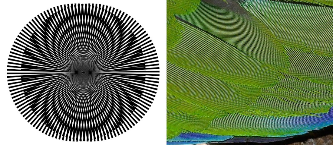
Figure E.1: Examples of Moiré patterns. Left: Curved Moiré pattern formed by two spoked wheels with different angular frequencies (image by SharkD, https://en.wikipedia.org/wiki/Moir%C3%A9_pattern#/media/File:Moire_Lines.svg). Right: Closeup image of parrot feathers (image by Fir0002/Flagstaffotos, https://en.wikipedia.org/wiki/Moir%C3%A9_pattern#/media/File:Moire_on_parrot_feathers.jpg).
E.1.2 The present study
In the present work, we attempt to reexamine the nature of the auditory system—whether it is continuous or discrete—at a fine-grained level of the sampling mechanism, should it exist. First, we hypothesize that if the auditory signal is discrete, then under some conditions it may be possible to evoke sensory aliasing. We assume that there is no such anti-aliasing filter in the auditory system. Using a psychoacoustic counting task, it is possible to elicit an audible confusion in the number of short events (sequences of two and three pulses), which suggests that aliasing may be at play. We infer from the results the bounds of the effective sampling rates of the system, using the Shannon-Nyquist limit. We use these results to estimate what sampling rates are possible under different conditions and find relatively high rates at onsets, which significantly drop after a few milliseconds. These patterns are in agreement with known neural adaptation patterns in the auditory nerve.
E.2 Experiments
A battery of several mini-experiments was administered in a single session that lasted about 45 minutes per subject. The results are reported as separate conditions of Experiments 1, 2 and 3, for clarity of presentation. The testing began with two training rounds that had the same structure as Experiments 1 and 3 (one round each, see below), but with correct / incorrect feedback for the subject. The testing order was set to Experiments 2, 1, 3, ending on the loud conditions of Experiments 3, 2, and 1 for half the subjects. The other half were tested on the loud conditions of Experiments 1, 2, and 3 first, and then on the normal-level conditions of Experiments 2, 1, and 3.
E.2.1 Experiment 1: Confusion between one, two, and three pulses
Introduction
While several studies have looked into the ability of listeners to differentiate between one and two pulses or clicks (Exner, 1875; Gescheider, 1966; Williams and Perrott, 1972), none to date specifically examined differentiation between two and three pulses. The distinction between the two sequence types is important, because both continuous (low-pass filtered due to a sliding temporal window) and discrete processing (aliasing) would give rise to confusion between two pulses and a single pulse. However, adding one more pulse to the stimulus affords a more critical benchmark to the discrete processing, aliasing hypothesis. With aliasing, three pulses can be confused with two pulses (three-to-two confusion), whereas the effect of a sliding window (continuous processing) is to smear three pulses into a single broad one, causing a three-to-one confusion. This is illustrated for some of the stimuli used in Experiments 1 and 2 in Figure §E.2, using approximate continuous temporal models and setting them to produce the most ambiguous output of a triple-pulse—one that might be confused with a double-pulse. In general, the output is either a smeared replica of the input, or a combined single large pulse, when the low-pass frequency cutoff is set sufficiently low and the sequence duration is short (See also Moore, 2013; p. 186, Figure 5.11).
An alternative to the simple sliding window models is to use a modulation filtering temporal model that is low frequency and relatively narrowband (Moore et al., 2009). This model can result in different pulse morphology due to filter ringing, which may be perceived as additional pulses in succession to the input pulses. With the correct timing of the ringing aligned with the periodicity of the pulse sequence, it may be interpreted as a double-pulse when the input is a triple-pulse (Figure §E.2, G) and as an irregular triple-pulse when the input is a double-pulse (Figure §E.2, F, H, and J). For these parameters, the single-, double-, and triple-pulses up to duration of 1.66 ms have almost identical morphology, of a single pulse followed by an additional low-energy pulse due to ringing. Pulse sequences of longer durations may sound ambiguous in terms of their numerosity, given their ambiguous morphology. For example, the 8 ms sequences (Figure §E.2, L and M) might appear as a quadruple-pulse for both double- and triple-pulse inputs, depending on how the extra ringing pulses are perceived / counted.
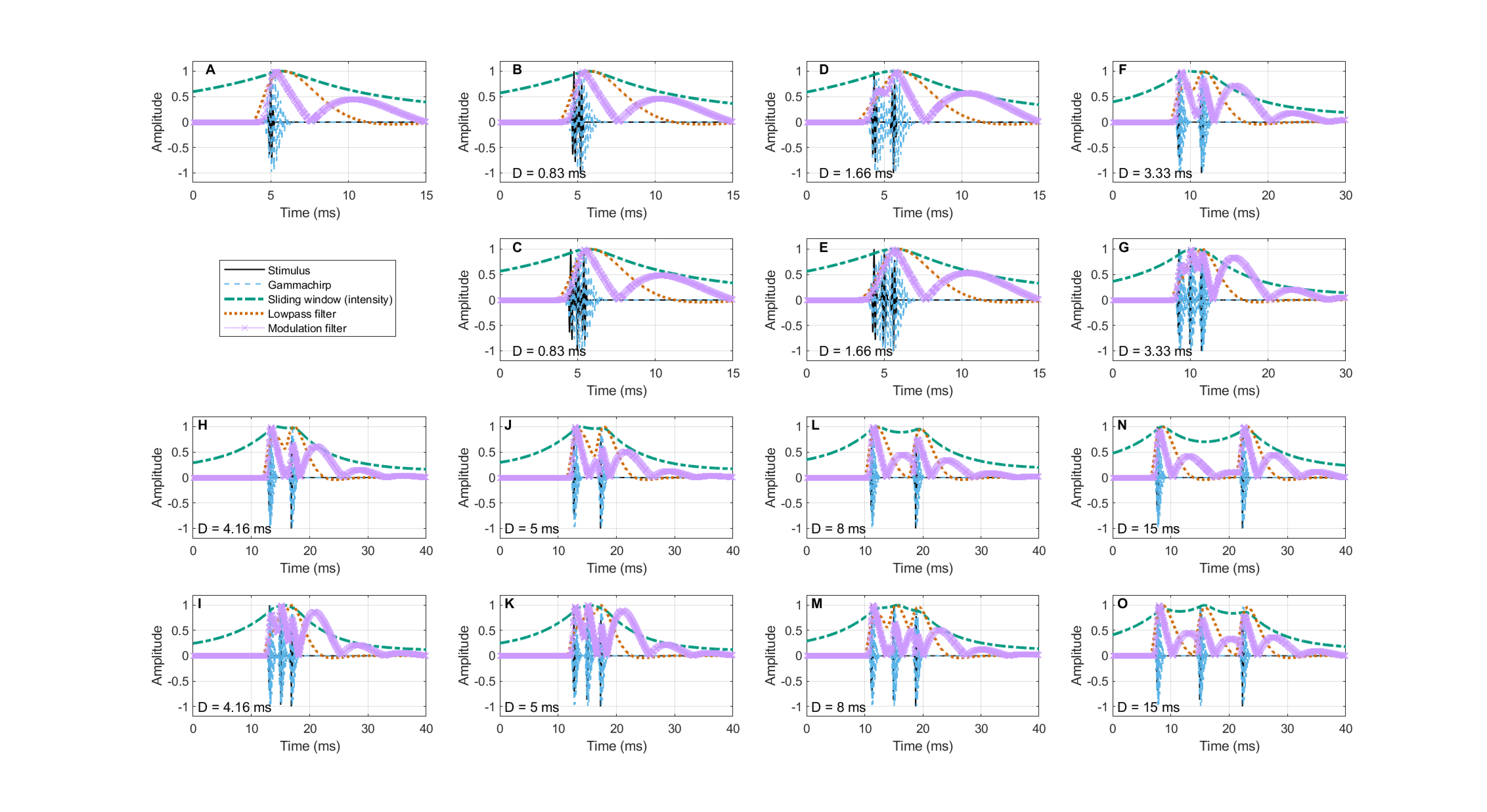
Figure E.2: The output of simple continuous temporal integration models of single, double, and triple Gabor pulse stimuli with 6000 Hz carrier and duration of \(W_p = 0.45\) ms per pulse, with seven total durations (0.83, 1.66, 3.33, 4.16, 5, 8, and 15 ms) of both double- and triple-pulse sequences are displayed in plots B–O. The original stimuli are plotted in black solid curves. The blue dashed curves show the output from a fourth-order level-independent gammachirp filter that models the band-pass filtering in the cochlea (Irino and Patterson, 1997) that is typically used as the first stage of temporal models. These filters can easily track the pulse envelope for the durations and carrier tested. The green dash-dot curves show the output of the sliding temporal window following an additional nonlinear stage, based on an asymmetrical round-exponential window parameters reported in Oxenham and Moore (1994). They show a smeared response that appears as a single broad pulse in all durations, perhaps with the exception of the longest pulse in plot N that can be interpreted as a double-pulse. The dotted red curves are the output following half-wave rectification, squaring, and low-pass filtering (fourth-order Butterworth with 100 Hz cutoff). The choice of low-pass cutoff frequency determines the degree of smearing in the output of the triple-pulse, which appears as a single-pulse in the shortest durations (plot B–E & G), ambiguous for some of the double-pulses (plots F, H–K & M), while it retains the pulse sequence shapes in the longer / slower sequences (plots L, N & O). The output of the half-wave rectified signal was also modulation-filtered (second-order Butterworth) and is plotted in purple crosses. These modulation-filtering parameters are based on Moore et al. (2009), using the minimum estimated center frequency (74 Hz, centered logarithmically) and a narrow filter (Q = 1.23), which produces noticeable ringing and gives rise to ambiguous patterns in several cases, including for the single pulse stimulus (plot A).
Assuming that a sampling mechanism is responsible for capturing all incoming sound, let the instantaneous sampling rate be \(f_s\). Using pulse trains as the simplest auditory multi-event available, let the pulse sequence periodicity be \(f_p\). The pulse sequence periodicity can be accurately sampled as long as \(f_p \leq f_s/2\), according to the sampling theorem (Shannon, 1948). If \(f_p > f_s/2\) then aliasing will occur, as higher frequencies will appear at lower sampled frequency than their continuous version (after reconstruction). This is illustrated in a cartoon example in Figure §E.3.
In the experiments below, the pulse sequence duration \(D\) is varied throughout the tests. In each sequence of total duration \(D\), either \(N=2\) or \(3\) pulses can be fitted, which determines the periodicity of the pulse trains. The threshold of aliasing can be estimated by the inequality
| \[ \frac{N-2}{D'} \leq \frac{f_s}{2} \leq \frac{N-1}{D'} \,\,\,\,\,\,\,\,\,\,\,\,\, N \geq 1 \] | (E.1) |
where the duration \(D'\) is the duration \(D\) corrected for the width of a single pulse \(W_p\) that is positioned at the end of the sequence, \(D' = D - W_p\). The larger the number of pulses per sequence \(N\) is, the more precise are the bounds that contain \(f_s\). However, it was determined in pilot testing that counting more than three pulses may be prohibitively difficult for untrained listeners, so in all the following experiments \(N \leq 3\).
In order to test the existence of aliasing, several psychoacoustic experiments were devised. The first experiment tested whether pulses with one, two, and three pulses (referred to throughout the text as single-, double-, and triple-pulses) are confused by listeners. The stimuli were pulses separated by silent gaps of different durations. Gabor pulses of constant carrier and Gaussian envelope were generated and employed to minimize the spectral and temporal smearing, by minimizing the uncertainty product of the very short signals (Gabor, 1946). Another condition was added with a higher carrier frequency, in order test whether the auditory channel center frequency has an effect on the observed sampling rate. The absolute level of the stimulus was modified in yet another condition. The motivation there was that the bandwidth of the auditory filters is known to increase as a function of stimulus intensity (Glasberg and Moore, 2000). This broadening should have a reciprocal effect in the temporal domain, making the sampling window narrower. The observed effect may be a sharper image of the pulses, where the gaps between them sound more distinct in case of near-aliasing at lower levels. Furthermore, it is known that the auditory nerve fires at a higher rate for inputs of higher intensity, at least when it is below its saturation level (Kiang et al., 1965; Liberman, 1978).
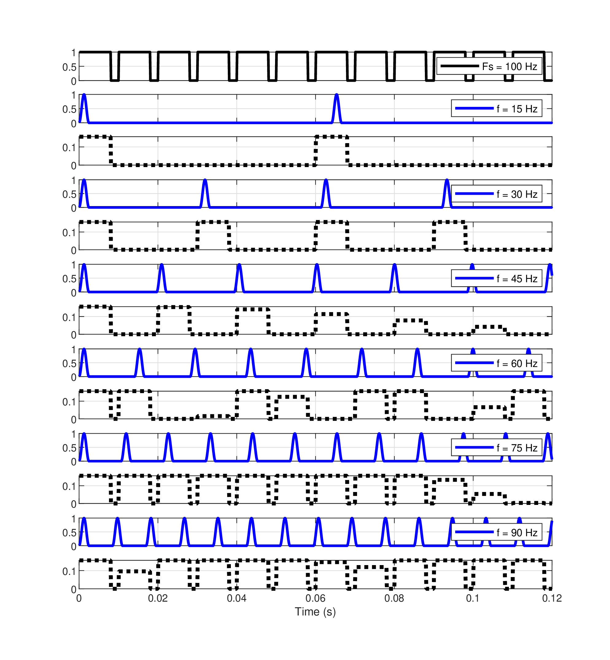
Figure E.3: A cartoon illustration of flat-top sampling (§14.4.3) using a 100 Hz sampling rate, and rectangular samples with 80% duty cycle (top curve in solid black). The input are pulse trains at rates of 15, 30, 45, 60, 75 Hz (in solid blue) and their sampled response are in dot black, which illustrates different degrees of aliasing. Frequencies below half the sampling rate show no aliasing, whereas the two highest frequencies exhibit some aliasing, as the signals are undersampled and folded downwards, giving ambiguous (and on average lower) frequencies than the input.
Methods
Subjects
Ten subjects with normal pure-tone audiograms (\(<20\) dBHL up to 8 kHz, recently assessed) participated in the study—3 female and 7 male, of 23–46 years old. All subjects participated voluntarily after the procedure was explained to them.
Setup
The experiment took place inside an anechoic chamber. A UFX RME sound card (RME Audio AG, Haimhausen, Germany) was used at a sampling rate 48 kHz. Stimuli were generated on MATLAB (The Mathworks, Inc., Natick, MA) and played diotically through Sennheiser HD-25 headphones (Sennheiser Electronic GmbH & Co. KG, Wedemark, Germany), which were calibrated using a G.R.A.S. Ear Simulator RA0045 (G.R.A.S. Sound & Vibration A/S, Holte, Denmark), connected to G.R.A.S. microphone preamplifier 26 AC, and Brüel & Kjær amplifier Type 2636 (Brüel & Kjær Sound & Vibration Measurement A/S, Nærum, Denmark). Calibration gains were found for tones of 6 and 8 kHz at 60 dB SPL (root mean square, RMS, levels), but were then multiplied by \(\sqrt{2}\) to determine a set value for the pulse amplitudes used in the experiment. The pulses of 6 and 8 kHz were level-equalized using these calibration values.
Stimuli
Double- or triple-pulse sequences were contained in an initial stimulus length of \(D=350\) ms, which could fit either two or three pulses. The pulses were 0.45 ms long (full-width half maximum), so they contained about three carrier periods of 6 or 8 kHz, regardless of the total stimulus duration (see examples in Figure §E.2). The stimulus level was 60 dB SPL and the 6 kHz stimuli were also presented at 80 dB SPL. As Gaussian pulses minimize the uncertainty relations of \(4\pi\Delta f \Delta t \geq 1\) (Gabor, 1946), the bandwidth of the pulse is about 338 Hz for both carriers. The carrier frequency was first generated for the entire stimulus duration before it was multiplied by the pulse envelopes (including the gaps), so to keep them in undisrupted phase at all onsets. This was found to yield continuous gap detection psychometric functions, as opposed to independent phase relations between pulses that made the psychometric function discontinuous (Shailer and Moore, 1987). In each test, single-, double-, or triple-pulse trains were presented in 13 fix total durations \(D\) that varied between 0.8–200 ms. The shortest nominal duration entailed that the pulses had no gaps between them, so that stimuli are approximately 0.4, 0.8 and 1.2 ms long, for one, two and three pulse-trains respectively. Obviously, the single-pulse stimuli were identical across the test, regardless of their nominal durations.
Procedure
Single-, double-, and triple-pulses were presented to subjects that had to determine how many pulses they heard by pressing the respective digit (1, 2, or 3) on the computer keyboard. Prior to the measurement, there was a training round with correct / incorrect feedback, which was eliminated in the actual test. The presentation order was randomized with respect to the gap and number of pulses, so that each subject was tested once on every number of pulses and duration (total of 39 stimuli per carrier and level condition per subject). Note that the subjects were tested multiple times on the same single-pulse, as it was identical across durations.
Results
The confusion matrix in Table §E.1 summarizes the results of Experiment 1. Four distinct patterns are apparent in the responses, which depend primarily on the duration of the sequences (marked with different shades of gray in Table §E.1). When the inter-pulse gaps (the quiet parts of the stimulus between the Gabor pulses) are long, perfect counting is possible with both 6 and 8 kHz carriers. This is the case for pulses that are separated by gaps that are 200 ms at 6 kHz, or longer than 75 ms at 8 kHz. Another response pattern occurs when double- and triple-pulses are confused more or less equally, but are not mistaken for a single pulse. For 6 kHz it happens most clearly between 15 and 3.33 ms, whereas for 8 kHz between 50 and 8 ms. However, hearing a double-pulse instead of triple-pulse becomes more common the shorter the stimuli are. For stimulus durations of 1.66 ms, listeners no longer perceived three pulses, and heard mostly a single- instead of a triple-pulse, although they did sometimes get the double-pulses right. Finally, at the shortest stimulus durations, 0.83 ms, all pulses tend to fuse into one (and indeed there are no gaps in the signal between the Gaussian pulses used here—0.83 ms was the duration of the double-pulse, whereas the triple-pulse was 1.2 ms long), so almost all responses were of a single-pulse. The 80 dB SPL condition data are very similar to the 60 dB SPL data, with a slight tendency for less double- / single- and triple- / single-pulse confusions, which is observed mainly in the short sequence durations of 1.66 ms.
| Pulses heard | |||||||||||
|---|---|---|---|---|---|---|---|---|---|---|---|
| Experiment 1 | Level Condition | ||||||||||
| 6 kHz, 60 dB | 8 kHz, 60 dB | 6 kHz, 80 dB | |||||||||
| \(D\) (ms) | Stimulus | 1 | 2 | 3 | 1 | 2 | 3 | 1 | 2 | 3 | |
| 200 | 1 | 10 | 0 | 0 | 10 | 0 | 0 | 10 | 0 | 0 | |
| 2 | 0 | 10 | 0 | 0 | 10 | 0 | 0 | 10 | 0 | ||
| 3 | 0 | 0 | 10 | 0 | 0 | 10 | 0 | 0 | 10 | ||
| 100 | 1 | 10 | 0 | 0 | 10 | 0 | 0 | 10 | 0 | 0 | |
| 2 | 2 | 8 | 0 | 0 | 10 | 0 | 0 | 10 | 0 | ||
| 3 | 0 | 1 | 9 | 0 | 0 | 10 | 0 | 2 | 8 | ||
| 75 | 1 | 10 | 0 | 0 | 10 | 0 | 0 | 10 | 0 | 0 | |
| 2 | 0 | 10 | 0 | 0 | 10 | 0 | 1 | 9 | 0 | ||
| 3 | 0 | 3 | 7 | 0 | 0 | 10 | 0 | 2 | 8 | ||
| 50 | 1 | 10 | 0 | 0 | 10 | 0 | 0 | 10 | 0 | 0 | |
| 2 | 0 | 9 | 1 | 0 | 6 | 4 | 0 | 9 | 1 | ||
| 3 | 0 | 2 | 8 | 0 | 1 | 9 | 0 | 4 | 6 | ||
| 20 | 1 | 10 | 0 | 0 | 10 | 0 | 0 | 10 | 0 | 0 | |
| 2 | 0 | 9 | 1 | 0 | 4 | 6 | 0 | 5 | 5 | ||
| 3 | 1 | 1 | 8 | 0 | 2 | 8 | 0 | 3 | 7 | ||
| 15 | 1 | 10 | 0 | 0 | 10 | 0 | 0 | 10 | 0 | 0 | |
| 2 | 0 | 6 | 4 | 1 | 7 | 2 | 0 | 4 | 6 | ||
| 3 | 1 | 2 | 7 | 0 | 3 | 7 | 0 | 3 | 7 | ||
| 10 | 1 | 10 | 0 | 0 | 10 | 0 | 0 | 10 | 0 | 0 | |
| 2 | 0 | 7 | 3 | 0 | 8 | 2 | 0 | 7 | 3 | ||
| 3 | 0 | 3 | 7 | 0 | 3 | 7 | 0 | 2 | 8 | ||
| 8 | 1 | 10 | 0 | 0 | 9 | 1 | 0 | 9 | 1 | 0 | |
| 2 | 0 | 6 | 4 | 1 | 2 | 7 | 0 | 8 | 2 | ||
| 3 | 0 | 4 | 6 | 1 | 4 | 5 | 0 | 1 | 9 | ||
| 5 | 1 | 10 | 0 | 0 | 10 | 0 | 0 | 10 | 0 | 0 | |
| 2 | 0 | 6 | 4 | 4 | 2 | 4 | 0 | 4 | 6 | ||
| 3 | 0 | 3 | 7 | 1 | 6 | 3 | 0 | 3 | 7 | ||
| 4.16 | 1 | 10 | 0 | 0 | 10 | 0 | 0 | 9 | 1 | 0 | |
| 2 | 0 | 7 | 3 | 3 | 5 | 2 | 0 | 8 | 2 | ||
| 3 | 0 | 4 | 6 | 3 | 2 | 5 | 1 | 4 | 5 | ||
| 3.33 | 1 | 9 | 1 | 0 | 9 | 0 | 1 | 10 | 0 | 0 | |
| 2 | 0 | 5 | 5 | 3 | 5 | 2 | 1 | 6 | 3 | ||
| 3 | 1 | 7 | 2 | 2 | 7 | 1 | 1 | 7 | 2 | ||
| 1.66 | 1 | 9 | 1 | 0 | 10 | 0 | 0 | 10 | 0 | 0 | |
| 2 | 7 | 3 | 0 | 9 | 1 | 0 | 4 | 6 | 0 | ||
| 3 | 9 | 1 | 0 | 9 | 1 | 0 | 4 | 5 | 1 | ||
| 0.83* | 1 | 10 | 0 | 0 | 10 | 0 | 0 | 10 | 0 | 0 | |
| 2 | 10 | 0 | 0 | 10 | 0 | 0 | 10 | 0 | 0 | ||
| 3 | 7 | 2 | 1 | 9 | 1 | 0 | 7 | 3 | 0 | ||
| Total | 1 | 128 | 2 | 0 | 128 | 1 | 1 | 128 | 2 | 0 | |
| 2 | 29 | 76 | 25 | 41 | 60 | 29 | 25 | 77 | 28 | ||
| 3 | 27 | 35 | 68 | 35 | 30 | 65 | 22 | 40 | 68 | ||
Confusion matrix of pulse sequences of variable durations (\(D\)) at 6 and 8 kHz and 60 dB SPL and 6 kHz at 80 dB SPL in Experiment 1. The number in each cell refers to the number of correct responses pooled over the 10 subjects (one condition per subject). *Note that the 0.83 ms stimulus contained no gaps between the pulses and was in fact 1.2 ms long in the triple pulse case.
It is possible to crudely estimate the duration thresholds between the double- and triple-pulses and between single- and double-pulses, at least in the duration ranges where only two responses were confused and were not contaminated by a third one. Using Eq. §E.1, it can be done by calculating the average between the two bounds in each duration point in the table that gives the individual sampling frequency. At 6 kHz, double/triple confusions begin to be common for durations between 5 and 8 ms, which gives effective sampling rates of 660 and 426 Hz, respectively. The confusions are virtually gone at 1.66 ms, which would have produced rates that are smaller than 2500 Hz. Similarly, the single/double confusion typically happens at around 1.66 ms, which corresponds to a 1250 Hz. These values are less distinct and longer in the 8 kHz stimuli, as they occur at 8–10 ms, corresponding to a sampling rate of 313–397 Hz.
Discussion
Experiment 1 revealed a confusion pattern that may be in line with a discrete processing, but can be contrasted with predictions from continuous temporal models. First, the results can be compared with the sliding window and low-pass filtering in Figure §E.2. The sliding window predicts that most stimuli of duration 15 ms or less would be perceived as a single-pulse or a double-pulse for the longest of these durations. This is clearly not the case, according to Table §E.1, which shows three-to-two confusions and not three-to-one or two-to-one confusions. Similarly, the low-pass filtering model predicts a single-pulse perception for stimuli of 5 ms or less, which is also not the case, as triple-pulses tended to be confused with double-pulses or identified correctly down to 3.33 ms. These models predict that the double-pulses would be correctly identified down to 3.33 ms and 4.16 ms. However, the observed identification rate of the double-pulses are not much better than the triple-pulses.
The modulation-band filtering model produces more ambiguous results that may coincide with the observed patterns. First, it predicts that stimuli of durations 1.66 ms or less would be perceived identically to a single-pulse, which appears as a double-pulse due to ringing (Figure §E.2). This is largely in accord with the results at the 60 dB SPL condition, whereas about half of the double-pulses were identified correctly at 1.66 ms at the 80 dB SPL condition. The pulse morphology predicted by the model at durations of 3.33 ms, 4.16 ms and 5 ms suggests that confusion between double- and triple-pulses may be possible, as was indeed the case in the results. With longer stimuli, the ringing appears more discernible, so that sequences may appear to consist of four or six pulses—answers that were not available as options in the alternative-forced choice test, even if listeners could hear and count them. However, if the ringing of the double-pulses at 3.33 ms and 4.16 ms could be indeed perceived as energetic enough to elicit confusions with triple-pulses, then one would expect such confusions to occur also between a single-pulse and a double-pulse, which was the case only in 1.5% of the responses, whereas the vast majority of the single-pulse responses were never confused. Therefore, although the modulation filtering model does give rise to a certain ambiguity that can account for several pulse confusion patterns, it is not internally consistent with the entirety of the patterns observed.
We note that the higher-frequency carrier measured (8 kHz) exhibited a lower and not as well-differentiated aliasing range as in comparison with the 6 kHz channel.
It is impossible to know what cues made subjects discriminate the pulse sequences, especially in the limit of a single fused event. Additionally, the precision of this test is low as far as the sampling rate estimation goes, given the non-adaptive method of measurement. If aliasing indeed exists, the individual threshold of sampling rate may be estimated more precisely using an adaptive method.
E.2.2 Experiment 2: Within-channel adaptive two-three numerosity threshold
Introduction
The confusion matrix from Experiment 1 revealed a broad range of effective sampling rates that may fit the aliasing working hypothesis. To determine the hypothetical sampling rate more accurately, an adaptive task was devised using the same stimuli for the double- and triple-pulses, but eliminated the option of a single-pulse. Hence, only one threshold at a time was explicitly tested here, instead of two.
The threshold was tested in four conditions. The first condition utilizes the same double- and triple-pulse stimuli as in Experiment 1, only with total stimulus duration that is set adaptively. It was implicitly assumed in Experiment 1 that the stimuli are narrowband, as the spectral splatter using the Gabor pulses is thought to be minimal because of their relatively small bandwidth and high carrier frequencies, which should confine the performance more narrowly to a single channel. However, in gap detection experiments, when continuous pure tones stop and restart abruptly, it creates a spectral splatter that has been sometimes masked with a notched broadband noise that occupies the adjacent channels, which ensures that the adjacent auditory bands to the carrier will have too low a signal-to-noise ratio to be capable of detecting the pulses in the flanks of their passband (e.g., Shailer and Moore, 1987). A similar argument for using such noise is that it reduces the availability of off-frequency listening (Patterson and Nimmo-Smith, 1980). Therefore, the second condition was set find out whether the high sampling rate estimates could be a result of integration of information over more than a single auditory channel. If this is the case, then a lower effective sampling rate may be measurable by masking the response of off-frequency channels using notched broadband noise. In the third condition, the carrier frequency of the pulses was roved within intervals. This was done in attempt to reduce some of the predictability that may characterize the stimuli, which could make the test easier by cuing the listener to a specific carrier frequency throughout the tested condition. It was hypothesized that a less predictable carrier may require extra vigilance from the system in order to sample the stimulus (possibly mediated by a top-down mechanism), which may putatively bring it closer to its maximum sampling rate capability. In the fourth condition, the stimulus was also presented at a level of 80 dB SPL to find out if there are any intensity effects that are more significant in an adaptive task, compared to those seen in Experiment 1.
Methods
Stimuli
The stimuli in the first condition were identical to those from Experiment 1. The complete pulse sequence was contained in an initial stimulus length of 350 ms, which accommodated either the double- or triple-pulse. In the second condition, the pulses were presented with notched noise that masks off-frequency channels. The noise was filtered with a third-order Butterworth band-stop filter that removed the energy at the same equivalent rectangular bandwidth (ERB) as the carriers (Glasberg and Moore, 1990). The noise RMS level was set at -40 dB from the pulse peak amplitude and its duration was either 50 ms, or 1.5 times the total stimulus duration—the longest of the two—and the stimulus middle was aligned with the middle of the masker. The relative level of the noise was determined in pilot testing so that discrimination was made more difficult, but the target still sounded clear. In the third condition, the carrier frequency was randomized around the center frequency of 6 kHz. Within each pulse sequence, the carrier was determined using a uniform distribution between 5495 and 6504 Hz, which corresponds to 1.5 times the ERB of the 6 kHz channel, according to Glasberg and Moore (1990). Therefore, no two consecutive pulses had the same exact frequency.
Procedure
Either a double- or a triple-pulse sequence was played at random and subjects had to determine whether they heard two or three pulses by pressing the respective digit key (2 or 3) in a single-interval two-alternative forced-choice (2AFC) task. An adaptive three-down one-up procedure was used, so that the stimulus duration was halved if the number of pulses were identified correctly three times in a row, but increased by half its duration for each incorrect response. The 79.4% threshold was determined after 14 reversals, by calculating the mean value of the last ten reversals (Levitt, 1971; Schlauch and Rose, 1990).
Results
All log-transformed data sets were successfully tested for normality using the Jarque-Bera test at the \(p>0.05\) level (Jarque and Bera, 1987).
The mean as well as the individual discrimination thresholds between double- and triple-pulse sequences are displayed in Figure §E.4 for the 6 and 8 kHz pulse sequences, along with their 95% confidence intervals. Sequences of mean durations of 14.2 ms at 6 kHz (95% CI [8.7, 23.0] ms) and 16.3 ms at 8 kHz (95% CI [10.0, 26.4] ms) were perceived correctly as containing either two or three pulses. On average, this is one event per 4.6–6.9 ms at 6 kHz, and 5.3–7.9 ms at 8 kHz. Note that the duration refers to \(D\) from Eq. §E.1, but the event rates were computed using \(D' = D - W_p\), to correct for the duration of the closing pulse in the sequence.
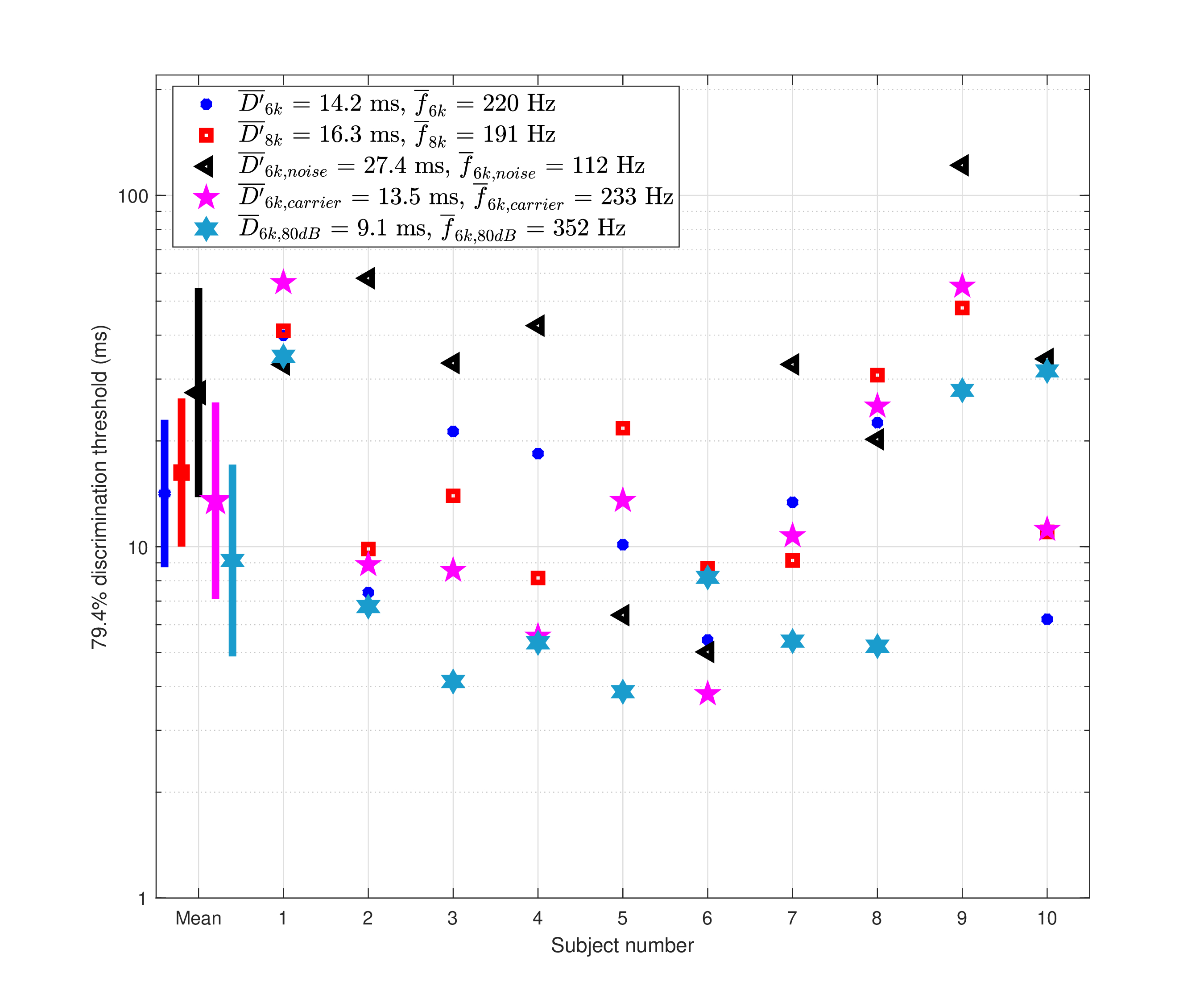
Figure E.4: Mean discrimination thresholds of double- and triple-Gabor pulse sequences for ten subjects (Experiment 2). The mean threshold values \(D'\) (the duration of the total stimulus minus the duration of one pulse) for the group and their 95% confidence intervals are displayed, as well as and the individual subject data. The 6 kHz thresholds are marked with blue asterisks and the 8 kHz with red squares. The broadband masking noise condition for the adjacent channels was added is indicated by black triangles. The roving carrier condition is plotted with magenta stars. The corresponding mean sampling rate estimates according to the bounds in Eq. §E.1 are given in the legend.
The sampling rate for each subject was calculated by plugging their \(D'\) threshold in the two bounds of Eq. §E.1, and the arithmetic average of the two was computed individually. Then, the arithmetic average of the individual rates was taken as the group sampling rate estimate. The 6 kHz pulses appear to have been sampled at a higher rate than the 8 kHz pulses—220 Hz (95% CI [133, 362] Hz) at 6 kHz and 191 Hz (95% CI [115, 314] Hz) at 8 kHz. The two rates are not significantly different, though, according to a paired t-test of the individual sampling rates (\(p=0.41\)). In the condition where off-frequency masking noise was added, there was a dramatic effect on the performance of six out of the ten subjects. The respective t-test comparison between the noise and no noise (randomized carriers) was significant (\(p=0.043\)). Additionally, the mean sampling rate in the noise condition dropped by almost 50% from the quiet condition to 112 Hz (95% CI [56, 224] Hz). In contrast, the roving carrier condition did not produce performance that was significantly different from the fixed carrier condition (paired t-test between sampling frequencies of fixed and randomized carriers gave \(p = 0.8\)).
Interestingly, the responses in the noise condition reveal two clear clusters: subjects whose temporal performance was unaffected by the noise (subjects #1, #5, #6 and #8) and all the rest, whose performance significantly deteriorated with the noise. The split in the performance was independent of the individual sampling rate baseline values in the quiet condition.
The high-intensity condition produced a sampling rate that was 132 Hz higher (352 Hz, 95% CI [180, 679] Hz) at 80 dB SPL than at 60 dB SPL, yet this difference was found insignificant according to a paired t-test (\(p = 0.19\)).
Discussion
The rates obtained in this adaptive test were lower (slower) than those estimated using the confusion matrix data of Experiment 1. However, the adaptive task produces the 79.4% threshold data, whereas Experiment 1 data that showed higher rates refer to the 50% threshold, so the thresholds in Experiment 2 are unsurprisingly higher.
We obtained a minimum temporal resolution threshold of 4.6–7.9 ms per event, which is higher than known broadband temporal acuity performance in humans, but is consistent with the sinusoidal gap detection 75% thresholds of about 5 ms (Shailer and Moore, 1987; Moore, 2013; pp. 200–201). The best performing subject's temporal threshold resolution of 1.6 ms was on par with the monoaural (broadband) resolution of 1.6 ms between one and two square 1-ms clicks reported in Gescheider (1966) and 1.66 ms gap detection between to 3-ms tones (Williams and Perrott, 1972).
The addition of noise had a much stronger effect on a subset of six listeners, but not on the other four. This clustering does not appear to be related to the baseline sampling rates without noise. However, it suggests that off-frequency listening may not necessarily be the cause for the apparent higher sampling rates obtained in the quiet condition, since four of the subjects had stable performances despite the noise. Alternatively, it can indicate that the six affected subjects had significantly broadened auditory filters at 6 kHz. While this seems improbable, it was not tested and cannot be ruled out.
Roving the sequence carrier did not cause a significant change in performance, which suggests that spectral predictability between intervals may not contribute much to the sampling rate values that were observed. Similarly, no level effects were found in this task, or any level effects were too small to produce significant results given the level difference (20 dB) and relatively low power of this experiment.
E.2.3 Experiment 3: The possibility of nonuniform sampling
Introduction
If the observations from the first two experiments reflect a physiological process in the auditory nerve or other auditory nuclei downstream, then we may expect to see adaptation effects as a result. Thus, we would like to find out if the results obtained in Experiments 1 and 2 can be generalized to longer sequences, or whether they represent rates that are too high to be sustained in more central nuclei that exhibit slower spiking rates (Joris et al., 2004). In other words, the observed responses may be relevant for the onset of the signals, but the corresponding rates may change later due to a nonuniform sampling strategy within the auditory system. The stimuli used in the first two experiments may have been short enough to always be processed as onsets by the auditory system. This may trigger adaptation effects in the auditory nerve, for example. On a higher level of processing, the listener knows that their attention is required for a brief moment at the onset, which may exert their finest detection capability only momentarily. Theoretically, an adaptive system may be geared to be frugal in its information processing resources (Weisser, 2018; pp. 143–162), so it may be designed to use a higher (or its highest) sampling rate just to monitor the stimulus onset. This can enable performance optimization on short temporal scales, similarly to improved spatial sampling in the central retinal areas in vision (Yellott, 1983). In contrast, if the system detects a stimulus that seems predictable beyond its onset, then a correspondingly unvarying (and maybe low) sampling rate can be generated that is sufficient to yield low resolution sampling of the input.
A possible issue with the regularly spaced pulse trains may be an exaggerated predictability between trials, since the context pulses are evenly spaced in a way that could be learned, possibly through a top-down effect. Thus, predictable stimulus rates may cause the system to produce sampling rates that are just fast enough for adequately sampling them, but not to spend more resources on higher rates. Jittering the pulse timing may further decrease their predictability. If the sampling rate set by the system is a result of predictability and not only of adaptation immediately after the onset, then reducing the stimulus predictability may coax the system to maintain a higher instantaneous sampling rate.
Methods
In order to test the hypothesis that the sampling rate can vary adaptively, the double- / triple-pulse confusion paradigm was repeated in a context of longer pulse trains. The stimuli were either evenly-spaced pulse trains, or they contained a triple-pulse sequence within the duration of a double-pulse (Figure §E.6, right). In other words, the pulse-sequence rhythm is momentarily disrupted, as a single pulse (the middle one of the triple-pulse) is presented at double the rate of the pulse train. The assumption here is that an evenly spaced pulse train can facilitate a timing prediction of when the next pulse should arrive after the onset. Thus, when the pulse train rate is half the instantaneous sampling rate of the system, a faster inter-stimulus pulse—hidden in between the regularly spaced pulses—may go undetected. Therefore, if the high temporal acuity performance of Experiments 1 and 2 were an onset-driven brief increase in the sampling rate, then the expected rate during a fast triple-pulse embedded in a slow pulse train context may be lower than when tested standalone, as in Experiment 2.
Procedure
Subjects were presented with two consecutive pulse trains and were asked to determine whether they are the same or different, by pressing a corresponding key. The two pulse trains were separated by the larger of a 450 ms gap or 1.5 times the duration of the pulse train. As in Experiment 2, a three-down one-up adaptive procedure was used with 14 reversals, from which only the latter ten were used for calculating the mean. The pulse train presentation was randomized with respect to whether they are two identical evenly spaced sequences that effectively contains a double-pulse (Figure §E.6), or one of the two contains a triple-pulse (Figure §E.6). Two conditions were administered with the different carrier frequencies of 6 and 8 kHz, each resulting in its own threshold. Two further conditions were administered where the pulse train was made more irregular both temporally and spectrally. This was done using randomized inter-pulse gaps (jittering), with and without roving carriers, as was tested in Experiment 2 for the short stimuli (§E.2.2). A final condition was repeated for the pulse train set at a higher level (80 dB SPL) than the standard presentation.
Stimuli
The pulses that were used to construct the pulse trains were identical to the ones of the previous experiments. The evenly spaced sequences contained eight pulses at 6 or 8 kHz (Figure §E.6, left). The odd sequence contains nine pulses: eight are identical to the evenly-spaced sequences, but another one appears exactly halfway between two pulses somewhere within the six middle pulses (Figure §E.6, right). Therefore, the double- or triple-pulse trains are inserted inside longer sequences of the same period as the double-pulse train. The position of the triple-pulse within the entire pulse train was randomized and could start anywhere between the second and the seventh pulse. To obtain jittering in the pulse train, the spacing between the pulses was randomized to be within \(\pm10%\) of its mean period value, following a uniform distribution. The roving frequency condition was generated using the randomized carrier frequencies as in Experiment 2, so that every pulse within a sequence had a somewhat different carrier frequency.
Results
The individual performances in all conditions are displayed in Figure §E.5, along with the main results from Experiment 2. The comparison between the pulse train and short stimuli reveals a noticeable drop in temporal acuity, confirmed by paired t-tests between the standalone sequences and those in the context of longer pulse trains are significant at the \(p<0.05\) level in both conditions (\(p=8\cdot10^{-5}\) for 6 kHz and \(p=5\cdot10^{-6}\) for 8 kHz). The mean sampling rates dropped by 3.4 times for the 6 kHz pulses to 65 Hz (95% CI [34, 122] Hz) and by 4.6 times on average for the 8 kHz pulses to 41 Hz (95% CI [33, 50] Hz) compared to the rates measured in Experiment 2. Despite some lowering of the thresholds of the pulse trains with jitter with and without frequency roving, there was no significant improvement in the sampling rate of either condition, as paired t-tests of data at the 0.05 level revealed (\(p=0.08\) for the jittered condition and \(p=0.52\) for the jittered and roving condition). The high-intensity condition produced a rate that was only 5 Hz higher for the pulse train sequence at 80 dB SPL than the 60 dB SPL condition (70 Hz (95% CI [36, 134] Hz)). This difference is insignificant using a paired t-test (\(p=0.77\)).
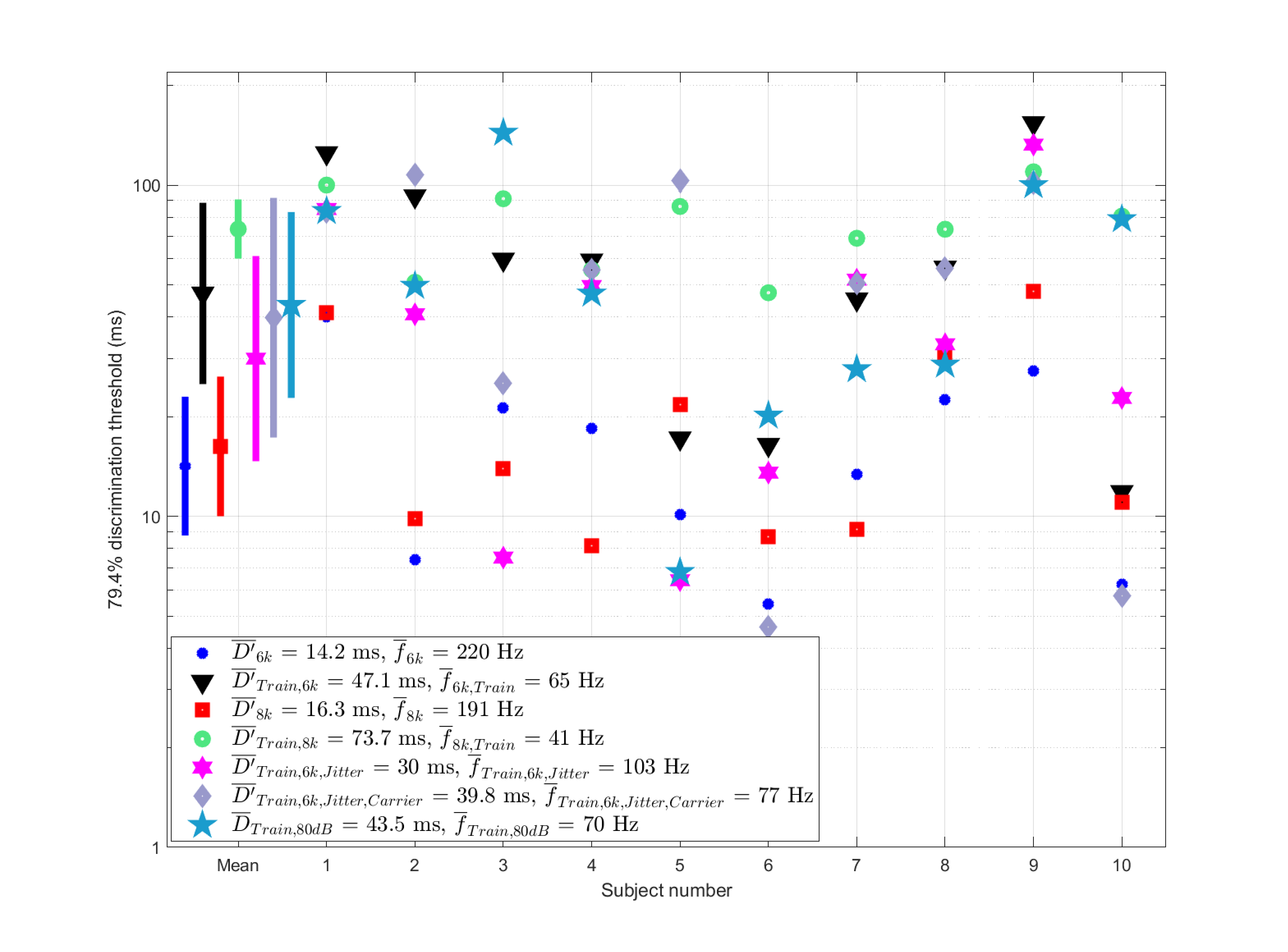
Figure E.5: Mean discrimination thresholds of evenly spaced pulse trains with a hidden pulse at 6 kHz (black triangles) and 8 kHz (green circles) carriers. The two conditions of jittered periodicity with and without roving carrier are shown in magenta stars and gray diamonds, respectively. For comparison, the thresholds of the standard double- and triple-pulse sequences from the previous experiment are shown in blue asterisks (6 kHz) and red squares (8 kHz). The group mean values include the 95% confidence intervals.
Discussion
When the (hidden) triple-pulse is inserted in a context of a periodic pulse train, no subject could discriminate the middle pulse out of the three as well as they did in the standalone condition of the same triple-pulse without the pulse-train context (Experiment 2). It suggests that the temporal resolution at the onset may be indeed higher than during the sequence. As before, we can compare the prediction of simple continuous models for the pulse trains at the thresholds achieved in the experiment or even lower. In Experiment 1, it was found that modulation band filtering can sometimes give rise to ambiguous outputs in terms of numerosity, albeit in an manner that is inconsistent with all the results. Since the thresholds in the present test are at least twice as high, there is no ambiguity that is implied by the modulation filtering model for a duration shorter (25 ms) than the threshold achieved in the best condition (30 ms), as can be seen in Figure §E.6 (bottom). A shorter duration stimulus of 12.5 ms yields something that may be considered morphologically ambiguous (Figure §E.6, top), which may have given rise to a “different” response in the test. However, the ambiguity is questionable in terms of its associated pulse numerosity.
If the results are instead interpreted as the output of a sampler with an adaptive sampling rate, then the triple-pulse can be thought to “fool” the sampler into missing a fast hidden event. An adaptation-perspective interpretation suggests that a prediction mechanism may be employed to detect the periodicity of the stimulus, which generates samples around the expected events. Alternatively, it could have merely been the effect of being far enough from the stimulus onset that led to lower-resolution sampling. A continuous model such as the one that was tested against above may have to include an adaptive stage with variable filter parameters in order to capture these results. A more surgical test that targets adaptation effects may require separating the placement randomization of the extra pulse to conditions of early and late placements, which may enable the analysis of the detection sensitivity decrease after onset.
Another alternative explanation of the data may involve forward masking by the initial pulses that has a cumulative effect by the time the hidden pulse appears. Such an effect is expected to be negligible because of the very short pulse duration, the fact that the pulses were presented at equal levels, and the fact that the thresholds of a couple of subjects changed relatively little as a result of the lengthening of the sequences.
Adding a subtle jitter to the pulse trains had an insignificant effect on the group level. It is possible that the jitter amplitude of 10% of the period was not large enough to elicit a substantial shift in performance. The addition of carrier roving did little to improve the performance and may have even canceled out the effect of jitter, just as Experiment 2 showed for the shorter stimuli. Unfortunately, the carrier randomization effect was not tested in a separate condition with the long pulse trains. Thus, the onset effect hypothesized may have been a more dominant factor than does a relatively small amount of jitter on listeners' temporal acuity.
It should be noted that the two tasks compared—one-interval forced choice in Experiment 2 and same-different in Experiment 3—are not identical and they may not be reflect the exact same psychometric function. The same-different task of Experiment 3 may have been more prone to response bias of the “same” type, which could have resulted in a worse sensitivity and therefore higher threshold—lower sampling rate (Macmillan and Creelman, 2005; pp. 217–218). Even then, however, the highly significant difference between the results of the two experiments seems to point at a true underlying difference.
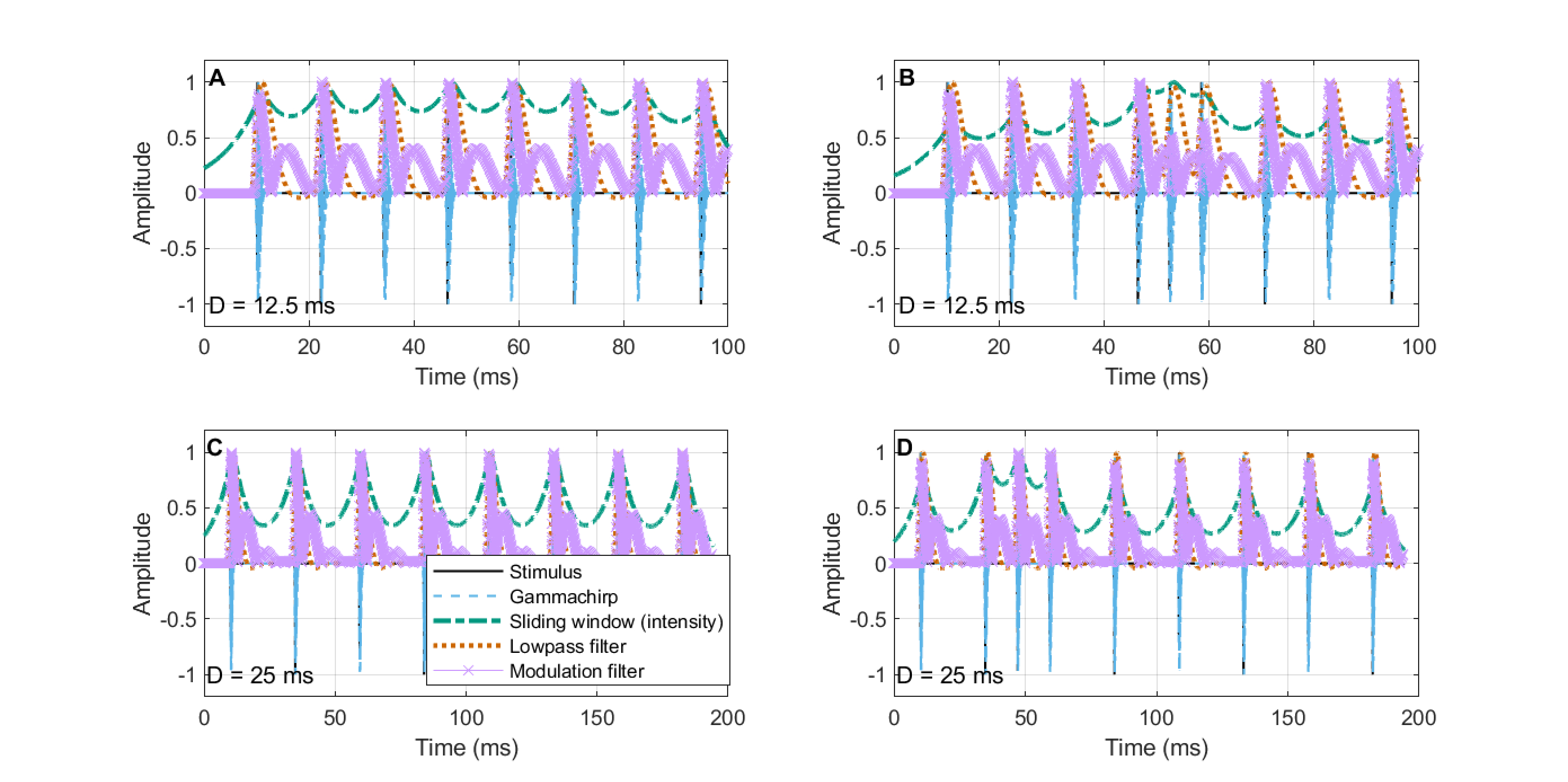
Figure E.6: Comparison of pulse train stimuli with hidden pulse of two durations of the pulse period: 12.5 and 25 ms. See Figure §E.2 for details about the models.
E.3 General discussion
In a series of experiments, the hypothesis of a discrete auditory sampling system was explored using adaptive and non-adaptive psychoacoustic methods. The resultant patterns are generally in agreement with theoretical predictions from temporally discrete auditory processing that includes adaptation effects.
E.3.1 Relationship to continuous temporal processing models
While we did not test against the continuous temporal auditory models specifically, we used them as conceptual benchmarks. As was illustrated in Figures §E.2 and §E.6, none of the continuous models can consistently describe our data. Application of modulation filtering was the only model that could sometimes give rise to ambiguity between double- and triple-pulses, but in a way which was inconsistent with the results of similar pulse morphologies, as well as with adaptive effects that can only be accounted for by dynamically changing the modulation filter parameters—something that was not attempted here.
We did not test the results against discrete auditory models, which were not formulated on sampling theoretic basis (see §E.1.1). Furthermore, the cited auditory models (both discrete and auditory) specifically tackled audibility thresholds, whereas the present study explored the perception of numerosity, which may or may not logically precede processing of long-term integration and loudness perception. Nevertheless, the results point to the validity of the general hypothesis of discrete auditory sensation, which has to give rise to sampling-theoretical artifacts like aliasing, in line with similar finding from vision (see §E.1.1).
E.3.2 Physiological correlates of the results
The physiological correlate of the auditory sampler has not been discussed in the psychoacoustic literature that hypothesized its existence (Viemeister and Wakefield, 1991; Patterson et al., 1992; Lyon, 2018), with the exception of Heil et al. (2017) that attributed it to general neural spiking distributions in the auditory system. The neural spike production in the auditory nerve is probably the most immediate candidate mechanism, since it is the first point of a discrete mechanism past the continuous cochlear mechanics.
The auditory nerve exhibits neural (spiking rate) adaptation, which may explain the difference between the responses to short pulse sequences and pulse trains. In general, onset response in the auditory nerve is characterized by a faster spiking rate (Galambos and Davis, 1943) and was recognized in early temporal models to be an important factor in modeling the temporal response of the system (e.g., Zwislocki, 1960). Rates that were electrophysiologically recorded in the auditory nerve of the gerbil are larger than those obtained here (Westerman and Smith, 1984). In the gerbil, a fast instantaneous rate (“the rapid component” that includes the initial 1 ms of the onset) was measured until about 10 ms from the onset and had an average rate of 642 spikes/s (Westerman and Smith, 1984). These values are almost three times faster than the 79.4% threshold of Experiment 2, and less than double those measured with 80 dB SPL pulses. They are within the range of the coarse double-triple threshold from Experiment 1. The next, “short-term”, component in the gerbil's response had a lower rate of 35-261 spikes/s—a broad range that contains the rates observed in the majority of the conditions in Experiments 2 and 3, with the exception of the 80 dB SPL short-pulse sequence measurement of Experiment 2 (Figure §E.4).
An alternative physiological correlate to the sampling operation is the T-Stellate type of neurons (choppers) that are mostly present in the cochlear nucleus (CN) (Oertel et al., 2011). The average spiking rates vary significantly between different cell types and as a function of level and frequency and can be several hundreds of spikes per second (Rhode, 1994), which may correspond to the observed rates here.
Both hypothetical correlates—the auditory nerve and the chopper cells—appear rather similar and it is possible that the chopper cells achieve downsampling, which means that the eventual perceived effect is a combination of both, and possibly further sampling units downstream.
One difficulty about using the neural correlates along with sampling theory is that spikes, in general, are not generated in the zeros of the incoming waves. However, sampling requires the generation of information also about low-level inputs, in order to be able to correctly reconstruct the arbitrary input. The sampling rate estimates were based on uniform sampling that includes the envelope zeros, contrary to normal auditory coding observations—it can be seen that any peristimulus spiking histogram traces the envelopes of periodic signals, but the spiking is distributed around the peaks (e.g., Heil, 1997). Mathematically, of course, it is necessary to distinguish between an interpolated (reconstructed) signal that is constant and one that is periodic, which can only be done by sampling at double the stimulus rate. It should be noted, however, that we used the sampling theorem assuming uniform sampling rate. Though, uniform sampling appears to be false in the auditory system for longer stimuli, so nonuniform sampling may have to be considered instead. Therefore, the computed sampling rates can only refer to instantaneous sampling rates, which could lead to instantaneous aliasing in the system.
In the motivation for the longer the pulse train stimuli in Experiment 3, we repeatedly invoked the design goal of making the stimulus less predictable, where the random appearance of the hidden pulse in the pulse train may have contributed to the lower observed threshold. However, the association of predictability with a low-level physiological correlate such as auditory-nerve or brainstem spiking rate adaptation may be controversial. Predictability in auditory processing—or rather, predictive coding that is geared to minimize uncertainty in future stimuli (e.g. Clark, 2013)—has been explored mostly in cortical processing and, to a more limited degree, in the midbrain and thalamus (Heilbron and Chait, 2018; Carbajal and Malmierca, 2018). While predictive coding is thought to be recurring hierarchically in the brain, a more localized relation between adaptation and predictive coding on the subcortical level (midbrain and thalamus) has only recently been proposed, but it was tested with stimuli that are up to two orders of magnitude longer than the stimuli we employed in the present study (Tabas et al., 2020; Tabas and von Kriegstein, 2021). Therefore, the interpretation we have provided here that ties together adaption and prediction may be considered speculative at present and has to be further investigated to find out whether it is warranted.
E.3.3 Individual variation and resemblance to informational masking
The large individual variability observed in all measurements suggests that the temporal properties of the auditory system may be age-dependent, learned, or dependent on other hidden parameters. The broad range of individual performances indicates that the auditory mechanics may be capable of transmitting the full information to the auditory nerve, but it may not always be processed with corresponding resolution in the central auditory circuitry. This may be a function of local neural circuits, of their instantaneous synchronization, or even of attentional resources that mediate early processing stages in the system.
The clustering into two subject groups according to their responses to the noise masker in Experiment 2 is reminiscent of the clustering observed in informational masking studies between “high-threshold” and “low-threshold” listeners (Neff et al., 1993). Approximately, only half of every random sample of test subjects (the high-threshold group) appears to be sensitive to informational masking effects, when the target is a tone that is masked by other tones that are well-separated in frequency. The masking remains high even when the separation is increased and is uncorrelated with the bandwidth of the auditory filter that corresponds to the target, when measured using a notched broadband noise task. Neff et al. (1993) suggested that the difference may be a result of different attentional filtering and is anyway not peripheral in origin. The main difference between this paradigm and the present study (Experiment 2) is that the masking noise was broadband and not tonal. Also, the task was temporal and not spectral. However, the explanation in which attention is divided in the subjects with high threshold in noise may work here as well, as it may seem improbable that the six other subjects all have broadened auditory filters.
An alternative explanation for this split in informational masking listener sensitivity was proposed in §15.4 based on coherent imaging theory. It was speculated there that the sensitivity to the kind of events that are normally presented as stimuli in informational masking tests (i.e., short tone bursts) may be interpreted by the auditory system as coherent noise, in analogy to speckle noise in optics (e.g., noise that appear like dust or small imperfections in the illuminated object). Then, the sensitivity may depend on the internal weighting of the auditory system to its coherent and incoherent images (roughly corresponding to the temporal fine structure and envelope processing, respectively) that makes the eventual perceived partially-coherent image. As the stimuli applied in the present experiment are of a similar nature to those found in informational masking studies, this explanation may apply here as well. Namely, listeners who tend to give higher weight to incoherent imaging are more affected by the masking noise that triggers a smoother listening, whereas listeners who give higher weight to coherent imaging do not smooth out the short speckle-like pulses.
E.3.4 No intensity effects
If there is a level effect at play on the temporal acuity of short pulse trains, then it may have to be revealed with more exhaustive testing, or at lower absolute intensity than was applied here. The auditory nerve spiking rate is also dependent on level, although it saturates at high levels (Kiang et al., 1965; Liberman, 1978). However, the higher rates measured at 80 dB SPL compared to 60 dB SPL (Figure §E.4) were insignificant in our study, which makes the direct link to the auditory nerve somewhat less certain. These presentation levels were chosen for comfort and audibility, before adaptation effects in the auditory nerve were considered from the results. Also, inasmuch as the change in the auditory filter bandwidth should have an effect on temporal acuity, the 20 dB input level difference may not be large enough to elicit it, and a larger difference in stimulus intensity may be required (Glasberg and Moore, 2000). Given the trend of the insignificant results from Experiment 1, it is possible that a test with higher statistical power could reveal an intensity effect.
E.3.5 Discrete or continuous sampling in the auditory system
Even after characterizing the auditory system input as sampled by an hypothetical adaptive detector, there would still remain many questions unanswered, should the system be understood more fully as a sampler. Some of these questions may be understood if the auditory nerve spiking is the responsible mechanism for sampling. For example, if hearing is discrete, then how are the samples triggered? Is there a regular clock, or an ad-hoc oscillator that triggers the sampling process? What is the sampling rate? Is it uniform or nonuniform? Other questions remain much more opaque: What is the shape of the sampling window? Is there a duty cycle? Are these parameters fixed or variable (i.e., adaptive)? Yet other questions require a more elaborate integration of the auditory system function: At what level(s) of the auditory system does sampling take place? Is reconstruction of the continuous signal from discrete samples a relevant concept physiologically and perceptually? If so, how and where are samples reconstructed to give the listener the experience of continuous perception? Are there any artifacts as a result of discretization and perceptual reconstruction (e.g., aliasing or spectral effects of windowing)? Can the processing be considered truly digital, once it is in discrete form?
E.4 Conclusion
The results from the above psychoacoustic experiments appear to reflect more closely well-studied features of the neural response to sound, which have not been directly integrated with behavioral data related to temporal acuity. Despite the wealth of knowledge about the nature of the auditory nerve and its coding, its sampling-theoretic considerations have been largely neglected, which means that any insights that may be garnered from sampling theory have been largely left uncharted to date. The above experiments were readily interpreted using a discrete sampling theoretic model that uses the notion of aliasing and non-uniform adaptive sampling rate, where the samples may have been triggered by the auditory nerve spiking.
Footnotes
188. Note that this conclusion is generalized here to the discrete model by Heil et al. (2017), as it shares a similar logic to the multiple-look model, although the examples below have not been tested against this more recent model.
189. Dithering is smoothing of sampling fluctuations, which are caused by the minimum quantization level (its finite resolution), through the addition of random low-level noise.
190. In system engineering, a well-designed analog-to-digital converter has to include an anti-aliasing (low-pass) filter, whose purpose is to remove high frequencies from the broadband input that are above half the sampling rate, which would otherwise be shifted downwards to frequencies within the passband, creating an aliased (and hence distorted) output (e.g., Proakis and Manolakis, 2006; pp. 389–391).
References
Amidror, Isaac. The Theory of the Moiré Phenomenon: Volume I: Periodic Layers, volume 38. Springer-Verlag, London, England, 2nd ed. edition, 2009.
Andrews, Tim and Purves, Dale. The wagon-wheel illusion in continuous light. Trends in Cognitive Sciences, 9 (6): 261–263, 2005.
Benedetto, John J and Teolis, Anthony. A wavelet auditory model and data compression. Applied and Computational Harmonic Analysis, 1 (1): 3–28, 1993.
Buus, Søren. Temporal integration and multiple looks, revisited: Weights as a function of time. The Journal of the Acoustical Society of America, 105 (4): 2466–2475, 1999.
Carbajal, Guillermo V and Malmierca, Manuel S. The neuronal basis of predictive coding along the auditory pathway: From the subcortical roots to cortical deviance detection. Trends in Hearing, 22: 1–33, 2018.
de Cheveigné, Alain. Pitch perception models. In Plack, Christopher J, Oxenham, Andrew J, Fay, Richard R., and Popper, Arthur N., editors, Pitch. Springer, 2005.
Clark, Andy. Whatever next? Predictive brains, situated agents, and the future of cognitive science. Behavioral and Brain Sciences, 36 (3): 1–73, 2013.
Dau, Torsten, Kollmeier, Birger, and Kohlrausch, Armin. Modeling auditory processing of amplitude modulation. I. Detection and masking with narrow-band carriers. The Journal of the Acoustical Society of America, 102 (5): 2892–2905, 1997a.
Dau, Torsten, Kollmeier, Birger, and Kohlrausch, Armin. Modeling auditory processing of amplitude modulation. II. Spectral and temporal integration. The Journal of the Acoustical Society of America, 102 (5): 2906–2919, 1997b.
Exner, Sigmund. Experimentelle untersuchung der einfachsten psychischen processe. Archiv für die gesamte Physiologie des Menschen und der Tiere, 11 (1): 403–432, 1875.
Gabor, Dennis. Theory of communication. Part 1: The analysis of information. Journal of the Institution of Electrical Engineers-Part III: Radio and Communication Engineering, 93 (26): 429–457, 1946.
Galambos, Robert and Davis, Hallowell. The response of single auditory-nerve fibers to acoustic stimulation. Journal of Neurophysiology, 6 (1): 39–57, 1943.
Gescheider, George A. Resolving of successive clicks by the ears and skin. Journal of Experimental Psychology, 71 (3): 378, 1966.
Glasberg, Brian R and Moore, Brian CJ. Derivation of auditory filter shapes from notched-noise data. Hearing Research, 47 (1-2): 103–138, 1990.
Glasberg, Brian R and Moore, Brian CJ. Frequency selectivity as a function of level and frequency measured with uniformly exciting notched noise. The Journal of the Acoustical Society of America, 108 (5): 2318–2328, 2000.
Heil, Peter. Auditory cortical onset responses revisited. II. Response strength. Journal of neurophysiology, 77 (5): 2642–2660, 1997.
Heil, Peter. Coding of temporal onset envelope in the auditory system. Speech Communication, 41 (1): 123–134, 2003.
Heil, Peter and Irvine, Dexter RF. First-spike timing of auditory-nerve fibers and comparison with auditory cortex. Journal of neurophysiology, 78 (5): 2438–2454, 1997.
Heil, Peter, Matysiak, Artur, and Neubauer, Heinrich. A probabilistic poisson-based model accounts for an extensive set of absolute auditory threshold measurements. Hearing Research, 353: 135–161, 2017.
Heilbron, Micha and Chait, Maria. Great expectations: Is there evidence for predictive coding in auditory cortex? Neuroscience, 389: 54–73, 2018.
Hofman, Paul M and Van Opstal, A John. Spectro-temporal factors in two-dimensional human sound localization. The Journal of the Acoustical Society of America, 103 (5): 2634–2648, 1998.
Hoglund, Evelyn M and Feth, Lawrence L. Spectral and temporal integration of brief tones. The Journal of the Acoustical Society of America, 125 (1): 261–269, 2009.
Irino, Toshio and Patterson, Roy D. A time-domain, level-dependent auditory filter: The gammachirp. The Journal of the Acoustical Society of America, 101 (1): 412–419, 1997.
Jarque, Carlos M and Bera, Anil K. A test for normality of observations and regression residuals. International Statistical Review / Revue Internationale de Statistique, 55 (2): 163–172, 1987.
Joris, PX, Schreiner, CE, and Rees, A. Neural processing of amplitude-modulated sounds. Physiological Reviews, 84 (2): 541–577, 2004.
Kelly, D. H. Flicker. In Jameson, Dorothea and Hurvich, Leo M., editors, Handbook of Sensory Physiology, volume VII/4, pages 273–302. Springer-Verlag Berlin, 1972.
Kiang, Nelson Yuan-Sheng, Watanabe, Takeshi, Thomas, Eleanor C., and Clark, Louise F. Discharge patterns of single fibers in the cat's auditory nerve. In Research Monograph No. 35. The M.I.T. Press, Cambridge, MA, 1965.
Kidd Jr, Gerald, Mason, Christine R, and Richards, Virginia M. Multiple bursts, multiple looks, and stream coherence in the release from informational masking. The Journal of the Acoustical Society of America, 114 (5): 2835–2845, 2003.
Kline, Keith A and Eagleman, David M. Evidence against the temporal subsampling account of illusory motion reversal. Journal of Vision, 8 (4): 13–13, 2008.
Levitt, H. Transformed up-down methods in psychoacoustics. The Journal of the Acoustical society of America, 49 (2B): 467–477, 1971.
Lewis, Edwin R and Henry, Kenneth R. Nonlinear effects of noise on phase-locked cochlear-nerve responses to sinusoidal stimuli. Hearing Research, 92 (1-2): 1–16, 1995.
Liberman, M Charles. Auditory-nerve response from cats raised in a low-noise chamber. The Journal of the Acoustical Society of America, 63 (2): 442–455, 1978.
Lyon, Richard F. Human and Machine Hearing. Cambridge University Press, 2018. Author's corrected manuscript.
Macmillan, Neil A. and Creelman, C. Douglas. Detection Theory: A User's Guide. Lawrence Erlbaum Associates, Inc., Mahwah, NJ, 2nd edition, 2005.
Moore, Brian CJ, Glasberg, Brian R, Plack, CJ, and Biswas, AK. The shape of the ear's temporal window. The Journal of the Acoustical Society of America, 83 (3): 1102–1116, 1988.
Moore, Brian CJ, Füllgrabe, Christian, and Sek, Aleksander. Estimation of the center frequency of the highest modulation filter. The Journal of the Acoustical Society of America, 125 (2): 1075–1081, 2009.
Moore, Brian CJ. An introduction to the psychology of hearing. Brill, Leiden, Boston, 6th edition, 2013.
Munson, WA. The growth of auditory sensation. The Journal of the Acoustical Society of America, 19 (4): 584–591, 1947.
Neff, Donna L, Dethlefs, Theresa M, and Jesteadt, Walt. Informational masking for multicomponent maskers with spectral gapsa. The Journal of the Acoustical Society of America, 94 (6): 3112–3126, 1993.
Oertel, Donata, Wright, Samantha, Cao, Xiao-Jie, Ferragamo, Michael, and Bal, Ramazan. The multiple functions of T stellate/multipolar/chopper cells in the ventral cochlear nucleus. Hearing Research, 276 (1-2): 61–69, 2011.
Oxenham, Andrew J and Moore, Brian CJ. Modeling the additivity of nonsimultaneous masking. Hearing Research, 80 (1): 105–118, 1994.
Packer, Orin and Williams, David R. Light, the retinal image, and photoreceptors. In Shevell, Steven K., editor, The Science of Color, pages 41–102. Elsevier, The Optical Society of America, Oxford, United Kingdom, 2nd edition, 2003.
Patterson, Roy D and Nimmo-Smith, Ian. Off-frequency listening and auditory-filter asymmetry. The Journal of the Acoustical Society of America, 67 (1): 229–245, 1980.
Patterson, Roy D, Robinson, K, Holdsworth, J, McKeown, D, Zhang, C, and Allerhand, M. Complex sounds and auditory images. In Cazals, Y., Horner, K., and Demany, L., editors, Auditory Physiology and Perception, volume 83, pages 429–446. Pergamon Press, Oxford, United Kingdom, 1992.
Penner, MJ. Persistence and integration: Two consequences of a sliding integrator. Perception & Psychophysics, 18 (2): 114–120, 1975.
Poeppel, David. The analysis of speech in different temporal integration windows: Cerebral lateralization as 'asymmetric sampling in time'. Speech Communication, 41 (1): 245–255, 2003.
Lopez-Poveda, Enrique A and Eustaquio-Martin, Almudena. On the controversy about the sharpness of human cochlear tuning. Journal of the Association for Research in Otolaryngology, 14 (5): 673–686, 2013b.
Lopez-Poveda, Enrique A. Why do i hear but not understand? stochastic undersampling as a model of degraded neural encoding of speech. Frontiers in Neuroscience, 8: 348, 2014.
Proakis, John G and Manolakis, Dimitris. G. Digital Signal Processing. Principles, Algorithms, and Applications. Prentice Hall Inc., Upper Saddle River, NJ, 4th edition, 2006.
Rayleigh, Lord. XII. On the manufacture and theory of diffraction-gratings. The London, Edinburgh, and Dublin Philosophical Magazine and Journal of Science, 47 (310): 81–93, 1874.
Rhode, William S. Temporal coding of 200% amplitude modulated signals in the ventral cochlear nucleus of cat. Hearing Research, 77 (1-2): 43–68, 1994.
Schlauch, Robert S and Rose, Richard M. Two-, three-, and four-interval forced-choice staircase procedures: Estimator bias and efficiency. The Journal of the Acoustical Society of America, 88 (2): 732–740, 1990.
Shailer, Michael J and Moore, Brian CJ. Gap detection and the auditory filter: Phase effects using sinusoidal stimuli. The Journal of the Acoustical Society of America, 81 (4): 1110–1117, 1987.
Shannon, Claude E. A mathematical theory of communication. The Bell System Technical Journal, 27 (3): 379–423, 623–656, 1948.
Simpson, William A, Shahani, Uma, and Manahilov, Velitchko. Illusory percepts of moving patterns due to discrete temporal sampling. Neuroscience Letters, 375 (1): 23–27, 2005.
Tabas, Alejandro, Mihai, Glad, Kiebel, Stefan, Trampel, Robert, and von Kriegstein, Katharina. Predictive coding underlies adaptation in the subcortical sensory pathway. arXiv preprint arXiv:2003.11328, 2020.
Tabas, Alejandro and von Kriegstein, Katharina. Adjudicating between local and global architectures of predictive processing in the subcortical auditory pathway. Frontiers in Neural Circuits, 15: 12, 2021.
VanRullen, Rufin, Zoefel, Benedikt, and Ilhan, Barkin. On the cyclic nature of perception in vision versus audition. Philosophical Transactions of the Royal Society B: Biological Sciences, 369 (1641): 20130214, 2014.
Viemeister, Neal F. Temporal modulation transfer functions based upon modulation thresholds. The Journal of the Acoustical Society of America, 66 (5): 1364–1380, 1979.
Viemeister, Neal F and Wakefield, Gregory H. Temporal integration and multiple looks. The Journal of the Acoustical Society of America, 90 (2): 858–865, 1991.
Warchol, Mark E and Dallos, Peter. Neural coding in the chick cochlear nucleus. Journal of Comparative Physiology A, 166 (5): 721–734, 1990.
Weisser, Adam. Complex Acoustic Environments: Concepts, Methods, and Auditory Perception. PhD thesis, Macquarie University, 2018.
Westerman, Larry A and Smith, Robert L. Rapid and short-term adaptation in auditory nerve responses. Hearing Research, 15 (3): 249–260, 1984.
Wever, Ernest Glen and Bray, Charles William. Present possibilities for auditory theory. The Psychological Review, 37 (5): 365, 1930b.
Wever, Ernest Glen. Theory of Hearing. John Wiley & Sons New York, Chapman & Hall Limited, London, 1949.
Williams, Kendrick N and Perrott, David R. Temporal resolution of tonal pulses. The Journal of the Acoustical Society of America, 51 (2B): 644–647, 1972.
Williams, David R. and Hofer, Heide. Formation and acquisition of the retinal image. In Chalupa, Leo M. and Werner, John S., editors, The Visual Neurosciences, volume 1, pages 795–810. The MIT Press, Cambridge, MA and London, England, 2003.
Wright, Beverly A and Dai, Huanping. Humans attend to signal duration but not temporal structure for sound detection: Steady-state versus pulse-train signals. The Journal of the Acoustical Society of America, 149 (6): 4543–4552, 2021.
Yamada, Walter Masami and Lewis, Edwin R. Predicting the temporal responses of non-phase-locking bullfrog auditory units to complex acoustic waveforms. Hearing Research, 130 (1-2): 155–170, 1999.
Yang, Xiaowei, Wang, Kuansan, and Shamma, Shihab A. Auditory representations of acoustic signals. IEEE Transactions on Information Theory, 38 (2): 824–839, 1992.
Yellott, John I. Spectral consequences of photoreceptor sampling in the rhesus retina. Science, 221 (4608): 382–385, 1983.
Zwislocki, J. Theory of temporal auditory summation. The Journal of the Acoustical Society of America, 32 (8): 1046–1060, 1960.
Zwislocki, Josef J. Temporal summation of loudness: An analysis. The Journal of the Acoustical Society of America, 46 (2B): 431–441, 1969.
de Cheveignè, Alain and Kawahara, Hideki. Missing-data model of vowel identification. The Journal of the Acoustical Society of America, 105 (6): 3497–3508, 1999.