Chapter 3

The acoustic source and environment

3.1 Introduction

Our sense of hearing is concerned much more with acoustic sources than with their reflections from the environment. This is in stark contrast to vision that primarily relies on optical images that are formed using reflected light from objects. Therefore, understanding the acoustics of typical sources in our living environment can potentially inform us about the type of signals that hearing has to deal with. However, much of hearing science was established using observations and insights obtained from a number of mathematically idealized and primitive stimuli that rarely (or never) occur in nature: pure tones, clicks, white noise, complex (harmonic) tones, and to a lesser extent, amplitude- and frequency-modulated tones. Judging from the prevalence of these stimuli in experiments in mammals (perhaps except for bats), it may be naively concluded that pure tones and harmonicity are common, that modulation is a relatively special feature in natural sounds, and that white noise is a common type of noise. The reality is not so clear-cut, though. Of course, nobody has made explicit claims that these stimuli are literally representative of realistic acoustics, and in fact, there has been a greater push in recent years for employing more complex stimuli and creating heightened realism in the laboratory. But the legacy of the mathematically simple stimuli still dominates the field.

The potential misrepresentation of the acoustic world in auditory experimentation is not the most problematic implication that these stimuli have on our understanding of the hearing system. Rather, it is the idea that signals can contain no modulation information. Real sounds have a beginning and an end, which means that they are modulated, even if the modulation appears extremely slow or aperiodic. Furthermore, in many signals, amplitude modulation and frequency modulation happen concurrently. Therefore, an acoustic source can become an object of hearing only through modulation—only by forcing it into vibration. Acoustic objects can become meaningful only if we consider these two necessary constituents of sound: carriers and modulators. Information transfer as sound requires both domains to be present.

The goal of this chapter is to provide a counter-narrative to the classical textbook approach of the ideal acoustic stimuli. At least a subset of the facts that are included in this overview are going to be familiar to readers with background in acoustics—only not in the way that they are brought together here. We will generally attempt to show that frequency is seldom constant, harmonicity and periodicity are rare, dispersion is common, and modulation of all kinds is ubiquitous. This will be illustrated using available examples from literature. After a short introduction that provides universally applicable tools to mathematically represent waves, the chapter proceeds to cover aspects of the acoustical sources themselves, as well as their acoustical environment. The conclusion is that the most general representation of a broadband acoustical sound is also the most suitable one: carrier waves modulated by complex envelopes. The changes incurred by the environment are most generally understood as changes to the complex envelope, but they may also lead to the stochastic broadening of the carrier.

3.2 Physical waves

Intuition into many fundamental problems in acoustics and hearing comes from linear wave theory and with it, Fourier analysis. Due to the equivalence between the spectral and the temporal domain representations, the linear perspective tends to be heavily reliant on the spectral nature of the solutions, which is most suitable for stationary signals. In reality, though, hearing deals with nonstationary signals. Using Fourier analysis, signals such as frequency-modulated tones that elicit pitch change over time, require broadband representations that do not correspond well to perceptual insight, even if they are mathematically correct (e.g., Blinchikoff and Zverev, 2001; pp. 383–395; see Figures §15.2 and §15.8 for examples of the Fourier spectra of frequency-modulated signals). This divide has required analytical tools that allow the spectrum to change over time, which were sometimes imported from time-frequency analysis or communication signal processing, and have been gradually incorporated and standardized in hearing theory. While this development enabled more freedom in accounting for the sensation of signals that vary both in frequency and in time, it has widened the gulf between classical acoustical theory, where much of the intuition lies, and the physical and perceptual reality.

This section relies heavily on an approach that was crystallized by Whitham (1999), but has antecedents in Havelock (1914) and Lighthill and Whitham (1955). We will use this approach to create a firm link between the signal representation that is more appropriate for temporal analysis and the acoustic waves in the physical world.

3.2.1 Linear analysis

Waves describe a very broad class of physical phenomena, which include acoustic, elastic, and electromagnetic fields, among many others. Incidentally, the simplest problems of these three fields are also described by the same hyperbolic differential equation—the homogeneous wave equation, which in three dimensions is

\[ \nabla^2 \psi - \frac{1}{c^2}\frac{\partial^2\psi}{\partial t^2} = 0 \]

(3.1)

where \(\nabla^2\) is the Laplacian operator, which in Cartesian coordinates and three dimensions is \(\nabla^2 = \frac{\partial^2}{\partial x^2} + \frac{\partial^2}{\partial y^2} + \frac{\partial^2}{\partial z^2}\). Then, \(\psi\) is some field function—e.g., pressure or velocity potential in acoustic waves, displacement in elastic waves, and electric and magnetic fields in electromagnetic waves. \(c\) is the propagation speed of the wave in the medium. A simple change of variables leads to the general solution of the wave equation

\[ \psi(x,t) = f(x - ct) + g(x + ct) \]

(3.2)

we use the scalar one-dimensional equation for simplicity, but the results are easily generalized to three dimensions. The solution is therefore a superposition of two waves going in opposite directions. In fact, these two waves are the solutions to simpler differential equations that can be obtained by factoring Eq. 3.1 into

\[ \left(\frac{\partial}{\partial x} - \frac{1}{c}\frac{\partial}{\partial t}\right)\left(\frac{\partial}{\partial x} + \frac{1}{c}\frac{\partial}{\partial t} \right)\psi = 0 \]

(3.3)

The forward-propagating wave is therefore represented by the second of these two first-order differential equations

\[ \frac{\partial\psi }{\partial x} + \frac{1}{c}\frac{\partial \psi}{\partial t} = 0 \]

(3.4)

A solution for this linear equation is

\[ \psi(x,t) = a e^{i(\omega t - kx)} \]

(3.5)

where the angular frequency \(\omega\) and the wavenumber \(k\) are real constants and the complex amplitude \(a\) are all determined by the initial and boundary conditions. It is implied that only the real part of the solution is used in physical problems, although the imaginary may be used just as well. From the solution, we have the speed of sound, or the phase velocity, which is defined as the ratio between the temporal (radial) and the spatial frequencies

\[ c = v_p = \frac{\omega}{k} \]

(3.6)

However, since the realistic physical medium in which the wave propagates is generally nonuniform, the phase velocity depends on the frequency. Then, as the spatial and temporal frequencies are interdependent, their relation can be expressed using either one of the two complementary forms of the dispersion relations²⁷

\[ \omega = \omega(k) \,\,\,\,\,\,\,\,\,\,\,\,\,\,\,\,\, k = k(\omega) \]

(3.7)

General solutions to the linear wave equation and related problems can then be obtained in the frequency domain using the Fourier integral, so that

\[ \psi(x,t) = \int_{-\infty}^\infty F(k) e^{i\left[\omega(k)t - kx \right]} dk \]

(3.8)

where \(F(k)\) is a function that can be determined from the boundary and initial conditions. This approach often results in series of solutions, or modes—each of which is associated with a specific combination of \(\omega\) and \(k\). The superposition of all the modes gives rise to the (full-spectrum) wave shape in the time-domain. Many of the famous problems in acoustics have been solved using this and related methods, which result in series of modes—sometimes with harmonic dependence.

When the propagation is composed of several waves of different frequency pairs \((\omega_n,k_n)\), it becomes meaningful to divide it into a fast-moving carrier and a slowly-varying envelope (or modulation). The simplest illustration of this procedure is given by the superposition of two waves of equal amplitudes and proximate frequencies, so that \(\omega_1 = \omega_c + \Delta \omega\), \(\omega_2 = \omega_c - \Delta \omega\), \(k_1 = k_c + \Delta k\), and \(k_2 = k_c - \Delta k\). The two frequencies beat as (Rayleigh, 1945; § 191)

\[ \psi(x,t) = a \cos(k_1 x - \omega_1 t) + a \cos(k_2 x - \omega_2 t) = 2a\cos(\Delta \omega t-\Delta kx )\cos(\omega_c t - k_c x) \]

(3.9)

The high-frequency part of the wave, the carrier \((\omega_c,k_c)\), moves at phase velocity, \(v_p=\omega_c/k_c\), whereas the low-frequency envelope moves at a velocity

\[ v_g(k) = \frac{\Delta \omega}{\Delta k} \]

(3.10)

where \(v_g\) is called the group velocity. In the limit of small frequency and wavenumber differences, \(v_g\) can be replaced with derivative

\[ \underset{\Delta\omega,\Delta k = 0}{\lim} v_g(k) = \frac{d\omega}{dk} \]

(3.11)

As it turns out, this definition holds in general and can be derived in a number of different ways and not necessarily through beating (Brillouin, 1960; Lighthill, 1965; Whitham, 1999).

In uniform, isotropic and linear systems, \(v_g = v_p\) and the system is dispersionless. More generally, though, all physical media are dispersive, so \(v_g \neq v_p\). As the shape of the wave propagation is determined by its envelope, it becomes distorted through propagation in dispersive media, as the different phases that give rise to the envelope shape become misaligned far away from the source of oscillation. Dispersive spatial and temporal effects are illustrated in Figures 3.1 and 3.2 for dispersion relations of the form \(\omega(k) \sim k^2\) and \(k(\omega) \sim \sqrt{\omega}\) that characterize vibrations in thin plates.

Dispersion and nonlinearities of the field give rise to more complex wave equations even in the simplest problems. For example, Eq. 3.4 becomes quasilinear as the velocity \(c\) is indirectly dependent on the field itself

\[ \frac{\partial \psi}{\partial t} + c(\psi)\frac{\partial\psi }{\partial x} = 0 \]

(3.12)

This equation applies to a wide range of wave problems that are not necessarily linear (or even directly relevant in acoustics). However, the concept of dispersion holds for all wave problems, including those that are represented by other differential equations. It can be shown that the dispersion relation of a problem contains the same information as in the differential equation itself.

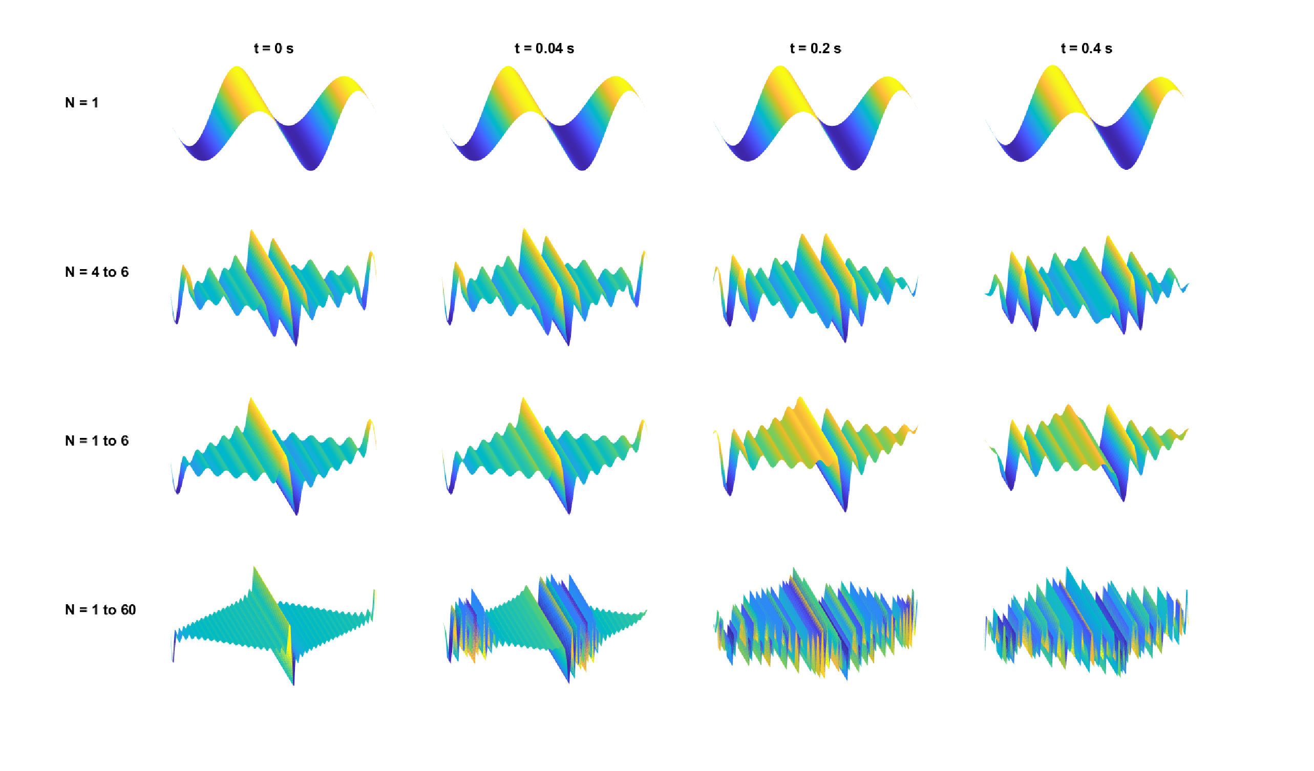
Figure 3.1: The effects of dispersion on the spatial acoustic field on (from top to bottom) pure tone, amplitude-modulated tone (200% depth), complex tone with six components, and a complex tone with 60 components. All components (marked with \(N\)) were summed with zero initial phase. Four conditions were computed corresponding to different time points measured in the same area, from left to right, at 0, 40, 200, and 400 ms. The dispersion relation is of the form \(\omega(k) \sim k^2\), which describes a thin plate (Fletcher and Rossing, 1998; pp. 76–77) set with the approximate properties of steel of 1 mm thickness, bulk modulus of 100 GPa, and density 8000 kg/\(\mathop{\mathrm{m}}^3\). The fundamental frequency is 100 Hz. All waveforms were normalized to maximum amplitude of 1, for clarity.

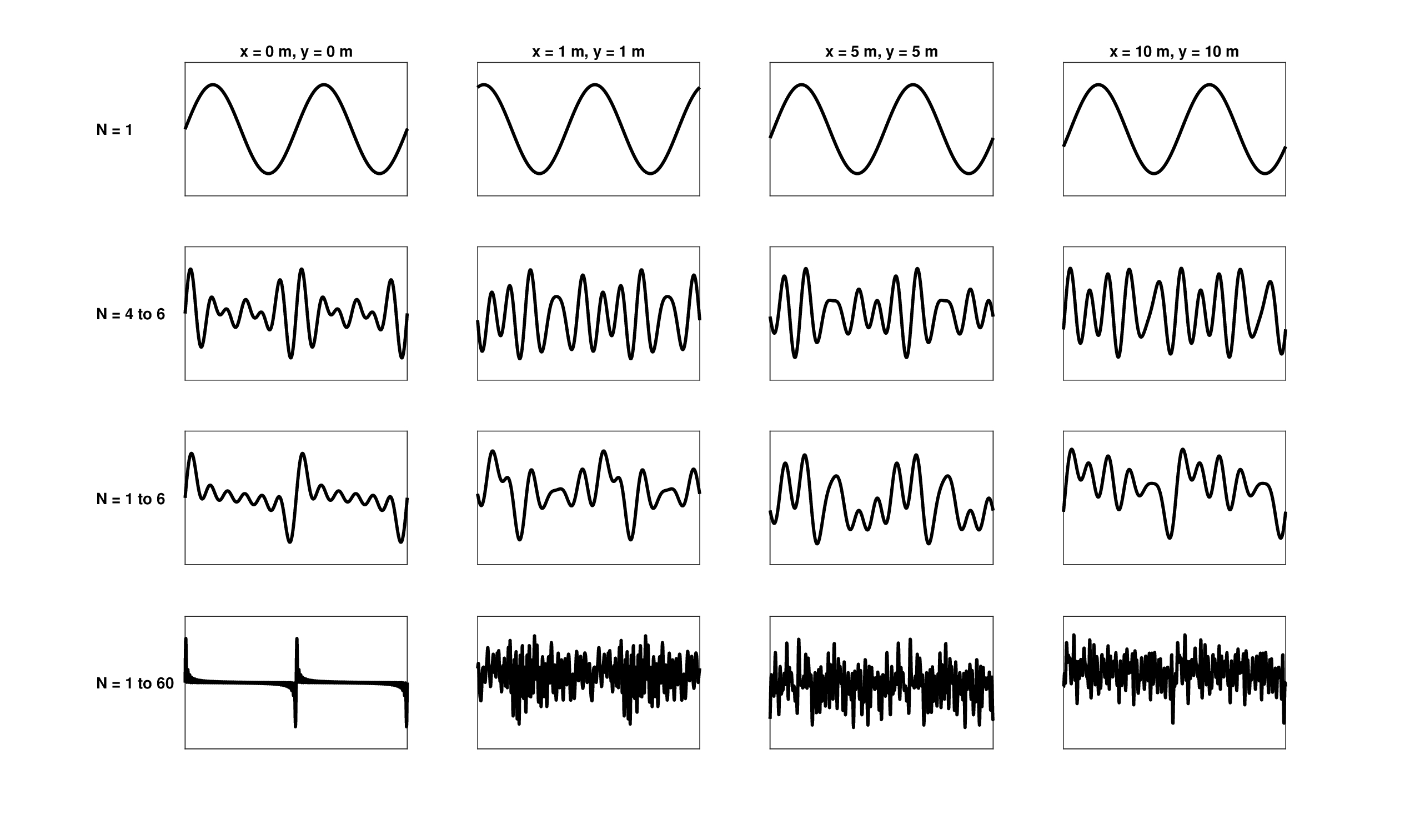
Figure 3.2: Similar to Figure 3.1, but displaying the time signal measured at different points on the X-Y plane. The dispersion relation of Figure 3.1 was inverted so that \(k(\omega) \sim \sqrt{\omega}\).

3.2.2 Dispersion analysis

While Fourier analysis is limited to linear systems, the concepts of dispersion and group velocity are applicable in nonlinear problems as well. A universal solution form, which is suitable for dispersion problems and for general nonlinear systems, allows both \(\omega\) and \(k\) to locally vary in space and time. Consider a wave that has a well-defined amplitude \(a(x,t)\) and phase \(\varphi(x,t)\) that can be expressed using

\[ \psi(x,t) = \Re \left[ a(x,t) e^{ i\varphi(x,t)}\right] \]

(3.13)

We consider solutions with a constant amplitude and a phase function that varies in time and space

\[ \varphi(x,t) = \omega t - kx \]

(3.14)

Differentiating the phase, we have

\[ k(x,t) = -\frac{\partial \varphi}{\partial x} \,\,\,\,\,\,\,\,\,\,\, \omega(x,t) = \frac{\partial \varphi}{\partial t} \]

(3.15)

Differentiating these expressions again yields

\[ \frac{\partial k(x,t)}{\partial t} = -\frac{\partial^2 \varphi}{\partial x \partial t} \,\,\,\,\,\,\,\,\,\,\, \frac{\partial \omega(x,t)}{\partial x} = \frac{\partial^2 \varphi}{\partial t \partial x} \]

(3.16)

Summing the two equations then results in

\[ \frac{\partial k(x,t)}{\partial t} + \frac{\partial \omega(x,t)}{\partial x} = 0 \]

(3.17)

Using the first dispersion relation in 3.7 with Eq. 3.17 gives

\[ \frac{\partial k(x,t)}{\partial t} + v_g(k) \frac{\partial k(x,t)}{\partial x} = 0 \]

(3.18)

where the dependence on \(k\) of the group velocity is now made explicit in \(v_g(k)\). We can also use the second dispersion relation in Eq. 3.7 to get a similar equation to 3.18 using \(\omega\) instead of \(k\)

\[ v_g(k) \frac{\partial \omega(x,t)}{\partial x} + \frac{\partial \omega(x,t)}{\partial t} = 0 \]

(3.19)

where the second term is the local frequency, frequency velocity, or frequency slope, which is introduced in Eq. §6.31 and is characteristic of frequency modulation. Equations 3.18 and 3.19 have the same form of the first-order hyperbolic equation as 3.12, although they were obtained in a different way. These equations take the universal form of conservation laws, which in this case was referred to as wave conservation by Whitham (1999). In analogy to other conservation laws, \(k\) can be thought of as the flow of the wave and \(\omega\) as its flux.

In dispersionless systems, the wave propagation is uniform and both \(k\) and \(\omega\) are space-invariant and time-invariant, so their partial derivatives in Eqs. 3.18 and 3.19 are zero and the equations become trivial. However, in dispersive media and nonlinear systems they convey information about the time dependence of the waves in the system, which may not be accessible using constant frequencies.

As the ears work largely as point receivers that detect acoustic waves that are one-dimensional throughout most of the audio range (see §11.2), signal processing of sound can factor the wavenumber \(k\) as a constant phase term, \(e^{ikx_0}\) at a point \(x_0\). In dispersionless systems, this phase is linear in frequency and produces a delay \(e^{i\omega x_0/c}\). Drawing from filter theory (Blinchikoff and Zverev, 2001; pp. 66–67), we refer to this phase as phase delay, which is generally given by

\[ \tau_p = -\frac{\varphi}{\omega} = \frac{k(\omega)x}{\omega} \]

(3.20)

for phase of the general form of Eq. 3.14 that excludes the usual \(\omega t\) term. In signal processing of time signals, the wavenumber \(k\) is not considered directly—only the frequency. In the present treatment, considering the spatial dependence too, results in \(\tau_p = x/v_p = t\) for a linear dispersionless system.

Similarly, it is also useful to quantify the deviation between the linear phase delay and any higher-order phase dependence on \(\omega\), which can be indicative of dispersion. Most generally, we define the group delay with respect to the phase as²⁸

\[ \tau_g = -\frac{d\varphi}{d\omega} \]

(3.21)

Using the same general phase and the dispersion relation of \(k(\omega)\) we get

\[ \tau_g = x\frac{dk(\omega)}{d\omega} = \frac{x}{v_g} \]

(3.22)

which can provide more insight if written as

\[ \tau_g = \frac{v_p}{v_g} t \]

(3.23)

Therefore, in the dispersionless case where \(v_g = v_p\), the group delay is equal to the phase delay, which is another way to say that the modulation that is being carried by the wave retains its shape—it is invariant to spatial and temporal shifts. In all other cases, the group delay quantifies the amount of dispersion, which grows the farther away the wave is from the origin and when the two velocities are markedly different. In normal dispersion (as opposed to anomalous dispersion) the group velocity is lower than the phase velocity, and we obtain a positive group delay (Brillouin, 1960).

The group delay is especially useful in a narrowband range of frequencies, for which the carrier and modulation frequencies are well-separated. With sufficiently narrow bandwidth, we are able to treat the group delay as approximately constant, even in dispersive systems. In broadband, dispersive media, and nonlinear systems, the group delay generally varies with frequency and becomes less linear the farther away it is from the carrier. This reasoning can be inverted and provide a useful operational definition for the rather vague “narrowband condition” that we highlight throughout §6: a narrowband range of frequencies is taken such that the group delay changes only a little from its mean value at the center frequency of the band (the carrier).

Note that if we let the phase be complex, this general wave analysis can be expanded to encompass the variable amplitude \(a(x,t)\) as well, which can be insightful in absorptive systems (Vakman, 1997). However, as most of this work is concerned with phase and dispersion, the explicit consideration of absorption will be relatively secondary.

3.2.3 Conclusion

This very brief introduction presents a universal approach to the representation of almost any wave, using a generalized phase function. Essentially, we have two approaches that hinge on the fundamentally different definitions for frequency that are discussed in §6.5.3—the Fourier frequency and the instantaneous frequency. The two are the same only in the simplest of cases, which can be considered approximately linear. Even if they yield mathematically identical solutions, each carries a different insight with it that may be incongruent with the other. When the acoustic system is nonlinear, but is still spectrally analyzed using Fourier analysis, we risk not only losing insight of the physics of the problem, but also downright misrepresenting its nature. Usually, the acoustic conditions are close enough to linear that we can retain a certain flexibility in switching back and forth between the Fourier and the instantaneous representations, depending on the problem. This will enable us to reexamine some of the familiar acoustic problems that are most relevant to our hearing world.

3.3 Acoustic sources

Three general mechanisms can cause acoustic wave generation in a closed region of fluid: solid body forces that create pressure gradients in the fluid, injection or removal of material from the region, and flow within the fluid that creates turbulence (Kinsler et al., 1999; pp. 140–142). Complex acoustical sources such as human speech may contain elements of all three. The few examples that are mentioned below are taken from the simplest and best studied sources, which illustrate that even simple acoustics is susceptible to “ill-behaved” phenomena that may be naively associated only with much more complex acoustics.

3.3.1 Primitive sound sources

Harmonic intervals are characterized by integer ratios of their constituent fundamental frequencies²⁹. The acoustic source itself may be considered harmonic if it produces an overtone series that is inherently harmonic (and hence periodic)—something that is captured in the popular complex tone stimulus. Such are the overtone series of the ideal string and the resonance series of the air column (pipe). However, arbitrarily shaped structures do not generally produce harmonic overtones when they vibrate. As harmony is a pillar of music that underlies consonance, it had to be progressively engineered into musical instrument design over generations. Therefore, the comprehensive analysis of acoustic sources in musical acoustics may be ideally-suited to identify “well-behaved” sources that have mathematically convenient properties such as harmonicity.

This section is heavily based on Fletcher and Rossing (1998), who systematically reviewed the physical acoustics of musical instruments. Many of the basic problems have been compiled by Lord Rayleigh (1945), but modern observations and modeling have considerably supplemented the classical (and sometimes idealized) solutions with a degree of realism.

Solid objects

Vibrating objects that are positioned in a fluid medium generate an acoustic field, which is determined by the object structure and its mechanical properties. The vibrations of solid objects can be shown to consist of normal modes of oscillation (also called eigenmodes), which are mathematically orthogonal (independent). Each mode is spectrally characterized by a natural frequency (also eigenfrequency) and, spatially, by a geometrical pattern of vibration (eigenfunction). Temporal characterization is divided into transient response (in terms of damping constant and decay time), and a steady-state time dependence that is generally taken to be sinusoidal. Depending on how and where the object is excited, combinations of the normal modes with different weights can be observed. Therefore, without loss of generality, the vibration of the object in the coordinate system of the object itself can be represented by

\[ \eta_{nml}(x,y,z,t) = \sum_{n=0}^{\infty}\sum_{m=0}^{\infty}\sum_{l=0}^{\infty}{a_{nml}\Psi_{nml}(x,y,z) e^{i\omega_{nml} t}} \]

(3.24)

where the displacement from equilibrium \(\eta\) varies in time and space, here in Cartesian coordinates. The most general case is given, which is three-dimensional with no special symmetry. Three degrees of freedom correspond to the three dimensions (e.g., of a thick plate), where each one is associated with an integer \(n\), \(m\), and \(l\). The eigenfunction is given by \(\Psi_{nml}(x,y,z)\) with its respective eigenfrequency \(\omega_{nml}\), which is factored into the steady-state harmonic dependence. The weight of each mode in the sum is given by the complex amplitude \(a_{nml}\).

Only systems with very simple geometries can be studied in closed-form—strings, bars, membranes, and plates are the primary ones among them. Typically, the normal modes of acoustic sources are studied spectrally—by noting prominent peaks in their spectrum—and mapping them to corresponding eigenfunctions. Most research characterizes the sources based on their steady-state response. Some instruments, such as the grand piano, have an idiosyncratic transient response that has been studied in depth, which showed the temporal envelope of each mode, as well as a distinct attack (onset) noise from the hammer action (Fletcher and Rossing, 1998; pp. 390–396).

The simplest vibrating solid object is the string. The ideal string is one-dimensional and its normal modes of vibration are exactly those studied by Pythagoras and found in the Fourier series solution of the string equation (Ibid., pp. 39–44). This string requires perfectly rigid support at its ends and zero bending stiffness. If these requirements are relaxed, the string overtones tend to deviate from harmonicity, as they are no longer integer multiples of the fundamental. So, if the end supports of the string can move, then the overtone series ratios become more compressed than the ideal integer overtone series (Ibid., pp. 52–53). Or, when the bending stiffness of the string (its two-dimensional cross-sectional elasticity) is taken into account, the overtone series become stretched (Ibid. 64–66).

The string can be mathematically extended into a two-dimensional thin bar or membrane. Like strings, bars vibrate harmonically in their longitudinal modes (Ibid., pp. 56-57), yet they vibrate inharmonically in their much more important transverse modes (Ibid., pp. 58–63). The ideal rectangular thin membrane also contains harmonic overtones, but they co-occur with inharmonic ones as well. If air loading, bending stiffness, or stiffness to shear is introduced to the membrane, or if the geometry is non-square (e.g., circular membranes) the overtone series can become completely inharmonic. Other shapes that have been modeled such as plates (thick membranes) and shells generally have inharmonic modes, even when their geometry is relatively symmetrical.

Modal dispersion

The dispersion of the normal modes is well-studied in many vibrating objects, which entails that the speed of vibrations in the different modes within the object depends on their respective eigenfrequency. Simple dispersive sources are the stiff string, the plate (Figure 3.1), and transverse waves in bars (Fletcher and Rossing, 1998; pp. 59–60, 65–66, and 77). Therefore, an envelope traveling within the vibrating object does not retain its shape in the object area and over time. The simplest case study for envelope dispersion is a single pulse, as its shape is dependent on the relative timing of the superimposed modes. This means that when an object is impacted—forced by an impulse somewhere on its surface, rubbed, broken, deformed—its response is not only affected by its unique vibrational behavior, but also by how and where it was impacted. As an impulse excites all modes in the structure, the transient pulse shape will necessarily depend on where it is measured in the field surrounding the object in the medium³⁰.

Resonators

Complex vibrating objects are often systems that consist of simple solid components, which are coupled to additional structures that vibrate and resonate. This coupling may accentuate and sometimes shift the modes of the standalone oscillator (Fletcher and Rossing, 1998; pp. 102–132). Many musical instruments employ resonant tubes and cavities, which are also commonly found in animal vocalization systems, and are of particular importance for modeling the vocal tracts of mammals and birds.

Pipes, like strings, are in good approximation one-dimensional at low frequencies where plane waves are the only normal mode that can propagate and carry sound in the pipe. An ideal pipe has a nearly harmonic series of resonances that depend on its length and termination (open or closed). The resonance frequencies tend to be slightly stretched due to reflections from the pipe ends that increase with diameter (Ibid., pp. 196–205). Other realistic deviations from harmonicity can take place when the walls of the pipe are not hard but yielding, which means that they have a finite (reactive) impedance (Ibid., pp. 202–205). Additionally, air has a finite viscosity near the walls, which causes viscous losses (mostly during flow) that affect the modes as well (Ibid., pp. 193–196). Also, thermal losses may be caused at the boundaries through compression, as the thermal conductance of the boundary material tends to be much higher than air (Morse and Ingard, 1968; pp. 290–292). Pipes shaped as conical horns can also exhibit nearly harmonic modes—in particular conical and compound (Bessel) shaped horns (Fletcher and Rossing, 1998; 216–218 and 461–464). At high frequencies, additional propagation modes can exist in the resonators (Morse and Ingard, 1968; pp. 492–498). Each mode has a cutoff frequency below which energy cannot propagate in the mode, as well as a characteristic spatial distribution and phase velocity associated with it, making the pipe dispersive.

Pipes have been mostly analyzed in the spectral domain, which provides steady-state solutions for harmonic inputs. The computation and measurement of transient signals is much more challenging and reports have been scarce. For example, a model of the attack transient of a flute (simple air column with holes) showed that it takes the instantaneous frequency about 5 ms to settle to a steady-state value to produce notes at 1000–1500 Hz (Keefe, 1990).

Mode-Locking

Despite the inherent inharmonicity of many of the vibrational systems mentioned, inharmonic modes can sometimes phase-lock to produce precise harmonic oscillations (Fletcher, 1978). There are several conditions that have to be met for this to take place. First, the modes have to be nearly harmonically related with simple ratios of small integers \(n/m\) (for \(n+m < 4\)). Additionally, the modes should be strongly coupled and driven in large amplitudes by a nonlinear force. These conditions are relatively restrictive and the prevalence of mode-locking in natural acoustic sources is unknown. Outside of the realm of musical instruments, mode-locking was measured in parts of the zebra-finch song, which suggests that the dynamics of their syrinx can be directly responsible for mode-locking (Fee et al., 1998).

Airflow generators

There are two primary airflow sound generation mechanisms that are employed in various musical instruments. The first is buzzing a valve (such as a reed or lips), as in saxophone, harmonica, and trumpet, as well as in the human vocal folds and the bird syrinx. As these generators are often coupled to an air column in a pipe, the combined system can give rise to harmonic sounds, which are excited by the nonlinear dynamics of the reed that modulates the airflow in the pipe (Fletcher and Rossing, 1998; pp. 418–424). The second mechanism generates jet airflow over a sharp edge as in whistles, flutes, and organs (Ibid., pp. 418–424). This mechanism is also nonlinear and is responsible for creating broadband noise when the jet flow is strong enough to cause turbulence, which is then shaped (filtered) by the resonances of the pipe (Ibid., pp. 528–529).

Stochastic sources

Completely fluid sound sources (e.g., water waves, waterfall, wind blowing) or those generated by large ensembles of similar units (e.g., walking on gravel, audience hum, rain) are very common and may also generate unique sounds (Schafer, 1994; pp. 158–160). These sounds are broadband and stochastic and do not have any stable vibrational modes that are associated with specific objects. Therefore, the analysis of turbulent and other complex sounds is generally done using stochastic tools (Morse and Ingard, 1968; pp. 768–772). Friction between objects is another common sound source that comes across as noise, although it may be a result of complex excitation of different harmonic modes that are generally not harmonic (Serafin, 2004). A qualitative taxonomy of everyday acoustic sources, based on their physical state and the type of force or function that excites them can be found in Gaver (1993).

3.3.2 Speech and other animal sounds

Human speech and animal vocalizations constitute complex acoustic sources that can be modeled as several basic components coupled together to generate sound. Two influential theories were developed with relation to human speech (vowel production, in particular). The most influential speech model is the source-filter theory (originally introduced by Chiba and Kajiyama, 1958/1942, according to Arai, 2004; Fant, 1970). It states that the harmonically-rich vocal-cord oscillations are independently shaped by the vocal tract resonances, which act as filters that endow the various vowels with their characteristic timbre. According to the myoelastic-aerodynamic theory, which complements the source-filter theory, sound is generated by aerodynamic energy that produces a jet airflow from the lungs and through the larynx, where it is converted to acoustic oscillations by the vibrating vocal cords (van den Berg, 1958).

Detailed mechanical and acoustical models have been further introduced to describe speech production acoustics. Stevens (1998, pp. 55–126) listed four specific mechanisms for sound production in speech—two of them were mentioned with respect to musical instruments—vocal-cord periodic modulations (similar to musical reeds), turbulence generation variations close to constrictions, sudden release of air from a pressurized cavity to the vocal tract (a short transient that is part of stop consonant production), and inward air suction using the tongue for constriction. The vocal cavities themselves are typically modeled as one-dimensional pipes with hard walls, where only plane waves can propagate. The associated filtering by the cavities is modeled as time-invariant linear functions, effective per specific articulation configuration. This configuration is determined by the size of the compartments (e.g, pharynx and the mouth cavity) and how they are connected among each other and to the nasal cavities. The specific resonances of the vocal cavities (formants) shape the rich harmonic spectrum coming from the larynx. The acoustic coupling between the different cavities, the effect of end-corrections, realistic wall properties, and perturbations to the cross-section of the pipes—all shift the resonances away from the natural harmonic series, although often not dramatically (Stevens, 1998; pp. 127–202).

Vocalizations of most mammals and birds are largely based on organs similar to humans, to the extent that the myoelastic-aerodynamic and source-filter theories can be applied just as well as they are for humans (Fitch and Suthers, 2016). There are also many exceptions, such as songbirds and toothed whales, which have a dual noise generation capability in their larynx/syrinx, and other animals that use highly nonlinear and even chaotic generation of sounds using the same mechanics (Fitch and Suthers, 2016; Herbst, 2016). Simpler animals like some anthropods can mechanically rub body parts to produce sounds (stridulation), whereas others like certain species of fish may not even be capable of producing sound.

The standard source-filter theoretical view of speech production has been challenged over the last decades, with the growing understanding that the transient nature of real speech signals cannot be satisfactorily accounted for by time-invariant linear filters (Teager and Teager, 1990). Nonlinear jet airflow speeds that were measured in the vocal tract suggested that vortices (turbulence) significantly contribute to the total speech energy, which entails a mechanism that is governed by the fluid-mechanics and not only by the acoustical dynamics (Teager and Teager, 1990; Barney et al., 1999; Shadle et al., 1999; Sharma et al., 2017).

3.3.3 Complex source modulation

The understanding of how the sound produced by acoustic sources is shaped would be incomplete without considering the role of modulation, which is known to be rife in natural sound sources, both as amplitude and as frequency modulations (Attias and Schreiner, 1997; Singh and Theunissen, 2003).

An important example of these effects has come to recent attention in speech modeling. In practical modeling of recorded speech signals, the inherent transience of real-world vocalizations is not adequately captured by any of the models mentioned in §3.3.2 (Sharma et al., 2017). From the signal perspective, animal (including human) vocalizations can be reduced to fundamental building blocks that vary dynamically: amplitude modulation, downward or upward glides (frequency modulation), broadband noise, constant (periodic) frequencies, and (near) pure tones (Klug and Grothe, 2010). Moody and Stebbins (1989) noted that when animals frequency-modulate their calls, it is always done gradually as a sweep and never in discrete steps. Species-specific vocalization systems have been shown to be matched by auditory systems that can be specifically tuned to receive the acoustic building blocks relevant to this particular vocalization, and thereby achieve processing efficiency (Casseday and Covey, 1996; Klug and Grothe, 2010; Theunissen and Elie, 2014). These sonic elements, at least in speech, are most effectively analyzed using time-domain methods that can extract the instantaneous envelope and frequency of the signals and avoid smearing effects that are involved in strictly frequency-domain methods (Huang et al., 2009; Sharma et al., 2017). Therefore, practical analysis of realistic speech applies somewhat generic solutions of time-frequency techniques, which decompose broadband signals to different modes that change in time—modes that are dynamically amplitude- and frequency-modulated (AM-FM). The superposition of all modes yields a representation of the complete broadband signal \(s(t)\) (Sharma et al., 2017)

\[ \hat{s}(t) = \sum_{n=1}^N a_n(t)\cos\left[ \omega_n t + \int_0 ^t m_n(\tau)d\tau + \varphi_n \right] \]

(3.25)

Here the speech signal is estimated as a multi-component signal of \(N\) modes, each of which has its own time-varying envelope \(a(t)\) and frequency \(m(t)\) and initial phase \(\varphi_n\). Ideally, the modes correspond to the harmonics and the formants of speech that are seen also in the static models (e.g., source-filter). In reality, determining the center frequencies \(\omega_n\) is the biggest challenge and different algorithms have been proposed to achieve it in the time-domain without resorting to Fourier analysis. Depending on the precise algorithm and signal, there may be a residual signal \(e(t) = s(t)-\hat{s}(t)\) that is not fully captured by the finite number of modes. However, in theory, the decomposition in Eq. 3.25 overcomes the situation caused by harmonic analysis that generates an infinite series of frequencies for every abrupt discontinuity in the signal³¹.

We recognize Eq. 3.25 as a summation of waves of the form of Eq. 3.13, which has time- and space- dependent amplitude and phase functions. While we did not deal directly with time-dependent amplitude in the discussion about dispersion above, it can be incorporated into the same framework if necessary by allowing the wavenumber \(k(\omega)\) to be complex. A case will be made later (§6.6.1) for employing a complex envelope as a catch-all modulation domain part of an arbitrary narrowband signal. This is a convenience that bundles the slowly varying AM and FM together along with a high-frequency and constant carrier. It is clear that the AM-FM modeling of speech can be applied using complex envelopes for the modes. In fact, the same procedure can be made to correspond to the generic sum of normal modes of Eq. 3.24, as long as the amplitude \(a_{nml}\) is made time-dependent in addition to being complex, \(a_{nml}(t)\). Of course, at the signal level, the factors that include spatial dependencies in Eq. 3.24 can be replaced by constants. The same goes for Eq. 3.25, which can be expressed using a complex envelope that includes both AM and FM.

There are several mechanisms that can constitute complex modulation in acoustic systems. The inclusion of these mechanisms in the complex envelope is a mathematical convenience, which does not change the physical signal. Three general categories of complex modulation are considered below. Note that in the hearing literature the category of spectral modulation is often invoked as one-half of the important spectrotemporal modulation. Spectral modulations can be the result of reflections that cause interference between the incident and reflected sounds. They are only mentioned in passing in §3.4.3.

Explicit forced modulation

The most obvious modulation is also unequivocally presented as such in literature. It is caused by setting the oscillator into vibration using a periodic external force. For example, according to the source-filter theory, the vocal folds modulate the airflow from the lungs at the fundamental frequency (Stevens, 1998). Additionally, the outgoing sound is temporally modulated by the tongue and lips, which also spectrally modulate the sound along with the other cavities in the vocal tract (Plomp, 1983). At much lower frequencies, the speech modulation spectrum is widely used in research, mostly referring to the natural amplitude modulation it has, which peaks at around 3–4 Hz (Steeneken and Houtgast, 1983) and is considerably diminished above 64 Hz (Drullman et al., 1994a; Drullman et al., 1994b; Singh and Theunissen, 2003). A vibrato (frequency modulation) effect in singing is caused by a periodic modulation of the fundamental frequency (Sundberg, 1995), similarly to vibrato in string instruments (Fletcher and Rossing, 1998; pp. 317–318). Also, string instruments (especially the viola and cello) are susceptible to the dreaded “wolf tone”, which is amplitude modulation caused by periodic low-impedance coupling between the string note and the normal mode of the instrument body (Fletcher and Rossing, 1998; pp. 312–313 and Chaigne and Kergomard, 2016; p. 629). Vibraphone notes can be amplitude-modulated (tremolo) upon periodically opening and closing its resonators using an electric motor (Fletcher and Rossing, 1998; pp. 638–639). As modulation that is not necessarily periodic, siren and guitar string pitch bending were given as realistic examples for frequency modulation in Schnupp et al. (2011, pp. 22 and 31), as are a few of the characteristic sound effects produced by the floating bridge and drum-head assembly of the banjo (Politzer, 2015). Finally, echolocating bats use frequency-modulated chirps as their main targeting signal.

Implicit modulation

Several types of signals that are sometimes seen as stationary are amenable to reformulation as modulated sounds.

The case of mode beating—the interference between two normal modes that are close in frequency—is somewhat problematic. Beating unmistakably behaves as amplitude modulation, but it lacks a physical carrier (Fletcher and Rossing, 1998; pp. 10 and 105). The standard mathematical solution is to set the carrier at the average frequency of the two mode frequencies with the difference frequency as the modulator (Eq. 3.8), although this description may not correspond to how the wave is generated at the source.

Constant tones are another common case. By making the carrier constant and assigning all the amplitude changes to the envelope, we obtain a very broad category of implicit modulations. They are typically overlooked or implicitly attributed to the carrier, despite the inherent ambiguity in this, as they can just as well belong to the envelope (see §6.6.1). A pure carrier is a pure tone—it has no beginning and no end—a precondition for keeping its frequency fixed. Therefore, sound onset and offset should count as a segment of a slow and long amplitude-modulated envelope, which includes the particular ramps associated with the onset and offset.

Nonperiodic changes in amplitude or frequency are also modulations, but with more complex envelope spectra that are not strictly sinusoidal or linear. In his landmark book about the source-filter theory, Fant (1970, p. 18) commented (emphasis in original): “The terms harmonic or periodic are not adequate, from a strictly physical standpoint. Because of the variations always present it would be more appropriate to speak of voiced sound as quasi-periodic.”

By including phase and frequency modulation effects, this category can be further expanded to all forces that cause some change to the otherwise static sound. For example, realistic vowel sounds contain fundamental frequency modulations (glides) that affect its formants before the vowel becomes static (Hillenbrand, 2013).

Transient response

Oscillators require a source of energy in order to vibrate. Sometimes it is provided from the outside by a distinctly separate object, and sometimes from within—in complex sources that have additional moving parts or internal sources of energy (e.g., a pendulum clock, a vocalizing animal, a fizzing chemical reaction). The mass, momentum, and material, as well as the area and duration of coupling between the force and the sounding mechanism affect the timbre of sound, often dramatically. Specifically when animal vocalizations (and human speech) are produced, they require coordinated muscle action, which may be periodic, impulsive, gradual, etc. and can instantaneously depend on numerous mechanical and aerodynamic factors in the system.

The solution to the inhomogeneous wave equation, which describes the forced source motion, contains two parts—a transient solution and a steady-state solution. The transient solution exhibits the normal modes of the oscillator, which inevitably decay. Each mode can be mathematically expressed as the product of a constant carrier and a decaying exponential envelope. The steady-state solution is caused by the external force. An external impulse reveals only the transient response, but all other forces produce more complex responses, which may involve dynamic frequency changes that can be incorporated into the complex envelope.

Another indirect modulation can take place if the source is moving while producing sound, which can create subtle frequency shifts through the Doppler effect (Morse and Ingard, 1968; pp. 699–700):

\[ f' = \frac{c+v}{\lambda} \]

(3.26)

where \(f'\) is the Doppler-shifted frequency for an object moving at speed \(v\) producing sound with wavelength \(\lambda\). Therefore, relative acceleration of the source or receiver can cause effective frequency modulation to a listener at rest. For example, an observer at rest, listening to a vocalization centered at 1000 Hz of an animal moving at an instantaneous velocity of 5 km/h will experience a maximum frequency shift of about 4 Hz. The modulatory effect on the spectrum and other room acoustic parameters that were produced in playing orchestral musical instruments, expressively (in motion), is documented by Ackermann et al. (2024).

3.4 The acoustic environment

The acoustic environment contains the medium for the radiated waves from the source. Given an arbitrary acoustic source, we would like to know how its sound is transformed by the time it reaches to a listener at a distance. As in the previous section, this review is highly selective and emphasizes acoustical effects that have received less attention in the context of hearing. The main focus is transient effects and how they distort the acoustic envelope through propagation in air, reflections, and various room acoustic effects³².

3.4.1 Radiation patterns

Vibrating objects of arbitrary geometrical shapes can produce complex radiation patterns in the medium, which determine the spatial distribution of the acoustic field (both pressure and velocity) away from the object (Morse and Ingard, 1968; pp. 306–394). In near-field, the radiation pattern may vary significantly as a function of position, especially if the source shape is not simple (i.e., if it does not possess any symmetry). Solid sources produce normal modes that vibrate with different amplitudes in different parts of the object geometry. Additionally, if the object is modulated by an external force, then their point of contact generally causes some normal modes to vibrate more than others. As most sources are inherently dispersive (§3.3.1), different elements of their external surface area tend to vibrate with slightly different phase, which varies as a function of frequency. Therefore, sources with multiple oscillating modes tend to sound different from different positions around them.

In farfield, the complexity of the acoustical radiation pattern may be reduced by approximating the sources to point size, or to other theoretically useful types of sources (e.g., dipole, spherical, line). This approximation dispenses with the precise object shape and replaces it with simpler and more symmetrical radiation patterns, compared to realistic conditions, in which arbitrary three-dimensional objects radiate asymmetrically. There is a practical limit to the usefulness of such approximations, as they tend to get too complex to derive much intuition from when higher-order terms are introduced (i.e., quadrapoles and higher-order terms than dipole). When this happens, the power spectrum of the source can be used alongside statistical tools to model the source radiation (Morse and Ingard, 1968; pp. 329–332).

Regardless of the specific geometry and modeling approach, many complex sound fields exhibit approximate plane wave behavior far from the source (i.e., when \(kr \gg 1\); see Table 3.1).

	Sound	Light
Field variables	pressure \(p\), velocity \(\boldsymbol{\mathbf{u}}\)	electric field \(\boldsymbol{\mathbf{E}}\), magnetic field \(\boldsymbol{\mathbf{H}}\)
Wave speed	\(c = \frac{1}{\sqrt{\rho \kappa}}\)	\(c = \frac{1}{\sqrt{\mu \epsilon}}\)
Characteristic impedance	\(Z_0 = \rho c = \sqrt{\frac{\rho}{\kappa}} \) (air)	\( Z_0 = \sqrt{\frac{\mu_0}{\epsilon_0}}\) (vacuum)
Scalar wave equation\(^\dagger\) (homogenous)	\(\nabla^2 p = \frac{1}{c^2}\frac{\partial^2p}{\partial^2t}\)	\(\nabla^2 E= \frac{1}{c^2}\frac{\partial^2 E}{\partial^2t}\), \(\nabla^2 H= \frac{1}{c^2}\frac{\partial^2 H}{\partial^2t}\)
Plane waves with solutions of the form \(\boldsymbol{\mathbf{F}}= F(\boldsymbol{\mathbf{k}} \cdot \boldsymbol{\mathbf{r}} - ct) + F(\boldsymbol{\mathbf{k}} \cdot \boldsymbol{\mathbf{r}} + ct)\)
Scalar field relations	\(p = \rho c u\)	\( E = \sqrt{\frac{\mu}{\epsilon}} H\)
Wave energy density	\(w = \frac{1}{2}\rho|u|^2 + \frac{1}{2}\kappa|u|^2 = \frac{|p|^2}{\rho c^2}\)	\( w = \frac{\epsilon}{2}E^2= \frac{\mu}{2}H^2\)
Intensity (energy flux)	\(I = cw = \frac{1}{2}(p^*u + pu^*) = \frac{|p|^2}{\rho c} \)	\(|S| = \sqrt{\frac{\epsilon}{\mu}}c w = \frac{\epsilon}{2\mu}E^2 = \frac{\mu}{2\epsilon}H^2 = \frac{1}{2}|E||H|\)
Far-field monopole (point source)
Scalar field	\(p = -\frac{i\rho ck}{4\pi r}S_\omega e^{i(\omega t - kr)}\)	N/A
Intensity (energy flux)	\(I_r = \frac{|p|^2}{\rho c} = \frac{\rho c k S_\omega}{4\pi} \frac{1}{r^2} \,\,\,\,\,\,\, I_\theta=I_\phi = 0 \)	N/A
Far-field dipole
Scalar field	\(p = -\rho c \frac{k^2 D_a \cos\theta}{4\pi r} e^{i(\omega t - kr)}\)	\(E = - \sqrt{\frac{\mu}{\epsilon}} c \frac{k^2 D_e \sin\theta }{4\pi r}e^{i(\omega t - kr)}\)
Intensity (energy flux)	\(I_r = \rho c \left( \frac{k^2 |D_a|\cos\theta}{4\pi } \right)^2 \frac{1}{r^2} \,\,\,\,\,\,\, I_\theta=I_\phi = 0 \)	\(I_r = \sqrt{\frac{\mu}{\epsilon}} \frac{c^2}{2} \left(\frac{ k^2|D_e|\sin\theta }{4\pi }\right)^2 \frac{1}{r^2} \)

Table 3.1: Comparison between the acoustic and electromagnetic analogous wave relations that are most relevant to hearing and vision, due to scalar fields and plane waves. Vector variables are printed in boldface. \(\boldsymbol{\mathbf{E}}\) is the electric field, \(\boldsymbol{\mathbf{H}}\) is the magnetic field, and \(D_e\) is the electromagnetic dipole strength. \(S_\omega\) is the acoustic point source strength and \(D_a\) is the acoustic dipole strength. The medium constants used are the fluid density \(\rho\), the adiabatic compressibility of the fluid \(\kappa\), the dielectric constant or permittivity \(\epsilon\), and the magnetic permeability \(\mu\), where in vacuum they are designated as \(\epsilon_0\) and \(\mu_0\). The intensity vector in electromagnetic theory is referred to as Poynting vector \(S\), but is called irradiance in radiometry. The standard medium is air for both sound and light, but in the case of light the values of vacuum are usually used instead as they are close enough to air. Because electromagnetic monopoles cannot be time-dependent (and there are no known magnetic monopoles), the simplest system that is directly comparable is a dipole in the far-field approximation. Naturally, its expressions are close to the acoustic dipole, which is less commonly used than the point source. The important thing to notice is that all source types have the same inverse-law dependence on distance in far-field (spherical divergence), up to scale constants. The acoustic expressions are taken from Morse and Ingard (1968, pp. 243, 258, 311–312) and the electromagnetic expressions from Born et al. (2003, pp. 15, 24–25) and Jackson (1999, pp. 410–413). Note that electromagnetic theory has multiple standardized normalizations, which means that similar equations often appear with slightly different coefficients, depending on the choice of units. See Jackson (1999, pp. 775–784) for further details. \(^\dagger\)In the context of acoustics, the homogenous wave equation applies both to the linearized elastic wave equation in solids and to the linearized acoustic wave equation in fluids, which are correct only for small amplitudes (Whitham, 1999; pp. 4–5). For a rigorous comparison of scalar and vector electromagnetic and acoustic potentials and fields (particularly geared for quantum mechanics), see Burns et al. (2020).

3.4.2 Acoustic information propagation in air

All material media exhibit acoustic dispersion and absorption, which affect the radiated waves in the medium and accumulates over distance (Brillouin, 1960). Absorption is responsible for dissipating acoustic energy through three primary mechanisms: viscosity, thermal conduction, and relaxation phenomena (causing molecular vibrations, rotations, ionization, or short-range ordering; Kinsler et al., 1999; pp. 210–241). At low frequencies, most mechanisms produce absorption that is quadratic in frequency, but this dependence can change as a function of the relaxation frequency of the gas, which in turn depends on temperature (and humidity, in the case of air). Absorption is associated with broadening of pulses on top of the spherical divergence attenuation of the wave (i.e., the drop in intensity as \(1/r^2\); see Table 3.1). In realistic conditions, though, the exact power-law of the frequency dependence may have to be determined empirically, as it can be a fractional power that is smaller than two (Treeby and Cox, 2010).

Absorption is always accompanied by dispersion, which causes pulse broadening as well as phase distortion that can lead to chirping. Unlike absorption, dispersion does not result in energy loss. The combined effect of dispersion and absorption is modeled using a complex wavenumber (e.g., Markham et al., 1951)

\[ k(\omega) = k_r(\omega) + ik_i(\omega) \]

(3.27)

where the real part \(k_r(\omega)\) corresponds to dispersion and the imaginary part \(k_i(\omega)\) to absorption. Importantly, the absorption and dispersion of \(k\) are not independent and the two form a Hilbert-transform pair. This is a result of the Kramers-Kronig relations, which connect the real and imaginary parts of functions in causal systems (Kramers, 1927; Kronig, 1926; Toll, 1956; Nussenzveig, 1972)³³.

The magnitude of the associated absorption and dispersion of the audio range in normal atmospheric conditions is small and is typically neglected in laboratory settings, except for large spaces or distances and high frequencies (Vigran, 2009; pp. 122–124). The most common analyses examine the effects of propagation of pure tones or broadband noise. Both types are stationary signals that do not provide much insight about the possible effects of the atmosphere on temporal modulation, which is a necessary element in acoustic communication³⁴. A more informative signal for this purpose is the pulse, which is transient and can be designed as narrowband (long duration) or broadband (short duration). A narrowband pulse moves in group velocity centered around its carrier frequency, whereas a broadband pulse (like a delta function) reflects more clearly the uniformity of the group velocity function in the medium, or the lack thereof. In any case, pulse propagation depends on the extent of the variations in the group velocity function, which are encapsulated in the dispersive properties of the medium. As the pulse shape is determined by the alignment of the phases of its spectral components, dispersion generally causes pulse deformation in propagation, to a degree that is proportional to the distance traversed (Vaĭnshteĭn, 1976 and §3.2.2).

Natural weather conditions entail fluctuations in temperature, density, medium velocity and scattering properties that make the atmosphere inhomogeneous and further affects the sound propagation. For example, it has been long known that sound propagation in fog causes attenuation in the outdoors (Tyndall, 1874; Cole III and Dobbins, 1970)³⁵ and also faster decay in closed rooms filled with smoke (Knudsen et al., 1948). Another important example is turbulent atmosphere that can be formed in windy conditions, which causes both pulse (temporal) and spectral broadening (Havelock et al., 1998). It is possible to get a handle on the magnitude of absorptive effects by evaluating the excess attenuation of the atmospheric absorption, which is estimated after subtracting the effect of spherical divergence loss of the signal (Wiener and Keast, 1959; Morton, 1975; Lengagne and Slater, 2002). The extent of this effect can vary significantly, as can be gathered from measurements of frog calls in a forest after rain (Penna et al., 2012), which revealed significant excess attenuation, while penguin calls in the dry and cold plains of Antarctica followed spherical divergence with no excess attenuation (Robisson, 1991) .

In this work we will be primarily interested in the quadratic frequency dependence (the curvature) of the dispersion (the group-velocity dispersion; see §10), whose small values are shown in Figure 3.3 for different distances in normal atmospheric conditions. Absorption effects are not studied directly in this work, but their potential role will be hypothesized at some points.

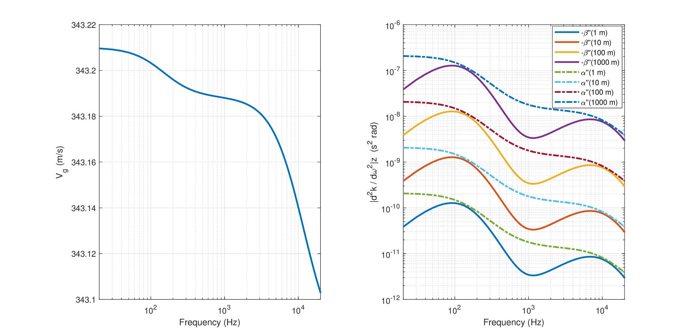
Figure 3.3: Sound propagation in air at \(20^\circ C\) and 50 % humidity, based on Álvarez and Kuc (2008). Left: Approximate group velocity is based on phase velocity of 343.21 m/s. Right: The absolute value of the (negative) dispersion and (positive) absorption curvatures (i.e., their quadratic frequency dependence). The dispersion was derived numerically from Eq. 9 in Álvarez and Kuc (2008). However, the same could not be done for the absorption of their Eq. 8 due to multiple sign reversals, but the trend was closely matched by dividing Eq. 8 by \(\omega^2\) to obtain the approximate absorption curvature.

3.4.3 Reflections

Apart from birds and bats in flight far from the ground, or animals in the depth of the ocean far from the ocean floor and water surface, all animal communication sounds are inevitably reflected from nearby surfaces—soil, rock, vegetation, or water. Theoretical reflection analysis ranges from simple to highly complex, depending on the amount of assumptions made about the reflecting boundary. As in propagation problems, much of the literature is concerned with pure tones and broadband noise, which model the effects of reflection on static amplitude or intensity, phase, and reflected angle. However, we continue to emphasize the effect of reflections on pulses and other transient signals that are more relevant for communication.

Several theoretical treatments of the reflection effects on sound pulses are found in literature. Pulses of arbitrary shape can be computed by convolving the impulse response function with a pulse of arbitrary shape (Morse and Ingard, 1968; pp. 259–270). The total field is a superposition of the incident pulse and a reflected pulse, which forms a wake of negative pressure. Depending on the delay between the incident and reflected waves, the two may interfere at the point in space and time of measurement and produce a deformed pulse. Another treatment of acoustic pulse reflection (and transmission) between two homogenous media was provided in Brekhovskikh and Godin (1990, pp. 113-125), where the reflected pulse is shown to be composed of a superposition of the incident pulse of and another pulse that is proportional to its Hilbert transform. In general, the reflection of a pulse by a realistic surface (of a finite acoustic impedance) causes deformation of the pulse shape. Hence, reflection can distort both spectral and temporal envelope, in a similar manner to dispersion (Brekhovskikh and Godin, 1990; p. 123). Most environments also contain objects of dimensions of the same order of magnitude as the sound wavelength that cause wave scattering, which is even more complex than simple reflection from large surfaces (Morse and Ingard, 1968; pp. 400–466). For a geometrical acoustical treatment of sound pulse reflection, see also Friedlander (1958).

Pulse deformation has been demonstrated in several measurements in-situ. For soil reflection, most measurements and applications rely on steady-state signals to evaluate the reflection properties, but in some cases pulses were used instead, which revealed severe pulse shape deformations following reflection (Don and Cramond, 1985; Cramond and Don, 1984). Reflection characteristics are sometimes known to be affected by surface waves at low heights over the ground (Daigle et al., 1996). In outdoor sound propagation, the acoustic impedance, porosity, and multilayeredness of different soils (e.g, grassland, sand, forest floor, porous asphalt) have been evaluated in several studies, and results were reproduced using different models of varying complexity (Attenborough et al., 2011). In underwater measurements, Cron and Nuttall (1965) showed that Gaussian and rectangular pulse-modulated pure tones become deformed as a result of reflections at angles greater than the critical angle (defined by the ratio of speeds of sound in the two media, water and ocean floor), when the pulse was relatively broad.

3.4.4 Room acoustics

An acoustic source radiating in a closed space produces numerous reflections between its boundaries. Other objects in the enclosure give rise to additional scattering that can be substantial. Also, in very large spaces, the atmospheric effects on propagation may be observable, especially as such effects accumulate with successive reflections. Therefore, depending on the complexity of the space, its dimensions, and its materials, we can expect that reflected pulses and other temporally modulated sounds may become severely deformed the farther they are in time and space from the sound at the source. Taking the sound field as a whole, it becomes gradually more diffuse the farther it propagates from the source and the longer it takes it to die out due to absorption.

Steady-state response

Two prominent approaches for the analysis of sound propagation in rooms exist in the literature—explicit wave equation solution for particular boundary conditions in one extreme, and a geometrical statistical approach in the other.

The first approach involves obtaining a closed-form solution of the wave equation with the boundary conditions of the enclosure, which yields a series of normal modes in three-dimensions (Morse and Ingard, 1968; pp. 554–576). The energy of any acoustic wave that propagates in the room has to be carried by its normal modes. This approach is insightful for large wavelengths (low frequencies) that are comparable with the dimensions of the enclosure. Solutions are generally interpreted in the frequency domain and relate to steady-state resonances, where each mode has its characteristic time constant for delay. At high frequencies, the increasingly high number of modes per unit frequency accounts for the erratic frequency response that rooms typically have (Lubman, 1968).

Geometrical acoustics, the second approach, employs idealized “sound rays” of negligible wavelength compared to the surrounding enclosure dimensions (Morse and Ingard, 1968; pp. 576–599; Kuttruff, 2017; pp. 81–102). A necessary condition for this to work is that the normal-mode density³⁶ is sufficiently high, so that an arbitrary frequency component can be carried by several normal modes simultaneously. This condition is generally fulfilled for sufficiently high frequencies (see §8.4.2).

The ability to use statistical methods opens the door for a practical definition of reverberation—the sound made by the ensemble of all the reflections. It is quantified by the reverberation time, which is defined as the duration it takes for a steady-state sound source that is switched off to decay by 60 dB (see §8.4.2). Its value depends on the room volume, the surface area of its boundaries, and their corresponding frequency-dependent absorption. While reverberation time is a temporal measure, it does not give sufficient information to infer the transient properties of ongoing nonstationary sounds.

It is often more practical to measure the room impulse response and extract different parameters from it, without having to make too many assumptions about the analytical problem (Kuttruff, 2017; pp. 193–218). This facilitates the separation of the direct and reverberant regions of the sound field. In the direct field region (measured by its distance from the source), the signal from the source is relatively intact and suffers the least deformation, as its level is higher than the field generated by the reflections—the reverberant field. The reverberant portion of the impulse response is typically separated to early reflections, which may be individually distinguishable as echoes, and to late reflections, which asymptotically behave as a statistical ensemble that is diffuse—it has a random phase function (Kuttruff, 2017; pp. 86–90).

Transient response

There are relatively few clear examples of temporal effects in room acoustics, beyond the obvious reverberant decay or distinct echoes in large spaces. Flutter echo may be the most familiar example—periodic reflections between parallel walls of long structures (like corridors) that are slow enough (longer period than about 25 ms) to be heard as temporal modulations—usually of low-frequency sounds (Kuttruff, 2017; pp. 90 and 167). More obscure effects include the chirping echo caused by diffraction from the stairs of the Mayan pyramid at Chichén Itzá in Mexico (Lubman, 1998; Declercq et al., 2004), or the sweeping echo following an impulse in some rectangular rooms (Kiyohara et al., 2002).

Note that shorter reflection periods than 20–25 ms can produce sound coloration (Atal et al., 1962), which is perceived spectrally rather than temporally (e.g., Rubak, 2004). In general, the interference between incident and delayed (reflected) wavefronts gives rise to spectral modulation, which can be measured with broadband sounds, and was demonstrated in a handful of natural sources in unspecified acoustic conditions (Singh and Theunissen, 2003), as well as for read speech (Elliott and Theunissen, 2009). The resultant interference, however, is never completely destructive in realistic conditions, due to the partial coherence between the incident and reflected waves (§8). Sinusoidal spectral modulation of the broadband sound are usually referred to as ripples in the auditory literature.

More mundane transient room acoustic effects exist as well. At low frequencies, the normal-mode density in rooms is relatively small, which can make specific modes stand out. For example, Knudsen (1932) demonstrated that even with a pure tone source in a small lightly-damped rectangular room of about 17 m\(^3\), low-frequency tones (around 100 Hz) changed their frequency during the decay, when they did not coincide with the frequencies of the normal modes of the room. Additionally, if the tone frequency fell between two modes, it exhibited noticeable beating, as its energy was shared between the modes. Similar phase and amplitude modulations obtained in tone decay with two, three, and four-wall structures (Berman, 1975).

In general, exact solutions of the room boundary condition problem lose their appeal at high frequencies, where numerous normal modes exist. Morse (1948, p. 393) suggested that for a pulse transmitted in a room to retain its shape, a large number of modes (\(>\)10) has to overlap with a pulse carrier. In contrast, an overlap of three modes only is considered sufficient to ensure a smooth response of steady-state sounds (Schroeder, 1996). As signals are generally not steady-state and can be highly variable, the realistic effect of reflections and reverberation can be more complex when it comes to transient signals.

In the reverberant field, the phase response of the room appears to be inconsequential, since listeners are able to detect phase differences only very close to the source and where the fundamental frequency is low, as measured with various broadband steady-state signals (Kuttruff, 1991; see also Traer and McDermott, 2016). Nevertheless, as is seen in §3.3.2, phase information is also necessary to appropriately reconstruct speech and other sound sources. Reverberation by its nature randomizes the signal phase when it is sufficiently far away from the source in time and space. The effect it has on transient sound may be appreciated from the modeling of the response to short Gabor pulses in two room geometries, which was found to be significantly closer to measurement when the complex acoustic impedance of the walls was included in the model (Suh and Nelson, 1999). While the basis of that model was geometrical, the complex impedance could propagate the (non-geometrical) effect of interference in successive reflections. In another study, it was demonstrated that the instantaneous frequency and amplitude of linear and sinusoidal FM signals become distorted in the room, when the involved modulation is fast relative to the inverse of the reverberation time (Rutkowski and Ozimek, 1997) .

With increasing reverberation, the sound envelope decays more slowly and can energetically mask subsequent sounds, if new sounds from the source are emitted before the decaying sound subsides. This effect is captured by the modulation transfer function (MTF) concept, which was imported into acoustics from optics, and has been used as a proxy to estimate envelope smearing effects (Houtgast and Steeneken, 1973; Houtgast and Steeneken, 1985). It is measured by applying sinusoidal amplitude modulation to bandlimited continuous noise bursts. The relative difference between the smeared output and the clean input can be averaged over all center frequencies for each modulation frequency band, typically of the range 0.25–16 Hz. In general, longer reverberation times decrease the received modulation depth (Schroeder, 1981), which entails a decrease in audible contrast between the high and low points of the envelope (§6.4.1).

An analogous measurement to the MTF in the transmission of sinusoidally frequency-modulated narrow noise bands (i.e., the center frequency of the noise band was frequency-modulated) was demonstrated by Rutkowski (1996). It was found that the frequency deviation of the modulation—analogous to modulation depth in AM—tends to decrease with higher modulation frequency and reverberation time, just like the MTF. However, in some carrier bands, the FM MTF was not monotonically decreasing and showed enhanced transmission.

It should be mentioned that the MTF, reverberation, and other room-acoustic principles do not apply only to closed spaces. For instance, sound propagation in a flat deciduous forest introduced significant amplitude modulation, attenuation, and reverberation in both pure and amplitude modulated tones (Richards and Wiley, 1980; see also, Padgham, 2004). It was hypothesized to have an impact on animal communication in these habitats, as vocalizations may have to be adapted to spectral windows where the information-distorting acoustics is minimal.

3.5 Transitioning from waves to stimuli

The previous sections made the case for high complexity of realistic acoustic sources and the various transformations that can befall them on the way to the receiver. In terms of analysis, it paints a somewhat bleak picture of acoustic waves that are not only complex right at their origin, but may also become hopelessly deformed in propagation. Such sources are a far cry from the popular and mathematically convenient pure and complex tones, and their environments are nothing like the safe acoustic spaces offered by the anechoic chamber or the audiometric booth. However, it is also evident that the direct sound path from the source to the receiver suffers the least deformation compared to longer acoustic paths due to large distances or multiple reflections. In closed spaces, where the direct and reflected fields are superimposed, there are additional issues of interference and signal-to-reverberation ratio, which make the direct field even more precarious than in the outdoors, where there are fewer reflections, typically.

As was argued in §1.3, hearing is primarily temporal, whereas many of the complications of realistic sources and fields manifest spatially. This means that the spatial dependence between two points can be generally reduced to a transfer function, while leaving any temporal effects explicit, as is customary in auditory signal processing³⁷. The difference is that we advocate for using instantaneous quantities (phase, frequency, and amplitude) throughout the signal representation, in order to be able to factor in all kinds of modulations, either inherent to the sound or as a result of its propagation.

We saw that a practical method—maybe the most practical method—to represent a complex signal like speech is by decomposing it to a sum of carriers with slowly-varying envelopes, which account for instantaneous changes both in amplitude and in frequency (if the envelope is allowed to be complex). We also know that the room acoustics and reverberation interact with the modulation domain, which should entail modulation deformation of some sort as well (usually a low-pass filtering of modulation frequencies). At the same time, the carrier domain becomes broader with accumulating dispersion and reflections, which leads to an overall loss of phase structure of the signal. However, even after transmission, the signal may still be representable as a component of a sum with slowly-varying complex envelope. In the direct field, the phase function and the exact frequency matter. In the reverberant field, the phase does not matter, and the sinusoidal carrier may have to be replaced with a stochastic carrier. In reality, neither the direct nor the reverberant fields accurately describe the acoustic field, which may be better understood as a mixture of both field types.

The distinction between the direct and reverberant fields has far-reaching implications for sound detection as is performed by hearing. Generally, the direct field provides a deterministic phase transfer function. To be able to make full use of the phase information, communication theory requires precise determination of the carrier frequency before demodulation (§5.3.1). Typically, it is achieved using phase-locking that synchronizes to the carrier. In reverberant fields and in the direct fields of random sources, the phase is random and demodulation can be applied much more simply to the intensity envelope only—no longer requiring phase-locking (which is anyway impossible when the phase is truly random). Both detection methods are useful for somewhat different purposes. We will later refer to the direct field as coherent, the reverberant as incoherent, and their corresponding detections as coherent and noncoherent. The process in which the phase of the direct field becomes randomized through reflections and reverberation will be called decoherence. These concepts are central in this work and will be explored from different perspectives along the subsequent chapters.

Footnotes

27. More precisely, Eqs. should be considered to be the dispersion formula, rather than the more general integral transformations that are implied by the dispersion relations and are due to causality constraints (Nussenzveig, 1972; footnote 13, p. 46).

28. For various derivations of this important formula, see Ville (1948) and Boashash (1992).

29. Note that the word “harmonic” is used in two related meanings in the wave physical literature. Harmonic dependence entails that the temporal dependence of the solution goes as \(e^{i\omega t}\). Harmonic intervals or sounds assumes that a few such solutions have natural frequencies that are related by integer ratios. In the present work, unless we refer specifically to a harmonic solution, harmonic should always be understood in the second meaning.

30. Interestingly, as noted by Brillouin (1960), dispersion in bars was analyzed first by Lord Rayleigh, which led him to formally talk about group velocity (Rayleigh, 1945; § 191), although the concept was originally introduced by William R. Hamilton (1839) without calling it by name.

31. The abrupt discontinuity can be modeled using a step function that modulates the amplitude of the signal. Using the standard Fourier-transform analysis, the step function \(u(t)\) has a hyperbolic continuous spectrum with an infinite support: \({\cal F}\left[ u(t) \right]= \frac{1}{i\omega} + \pi\delta(\omega)\).

32. A few audio demos that demonstrate the aggregate effect of some of the phenomena that are discussed in this section are provided in /Section 3.4 - Radiation, dispersion, reflection, and reverberation/. The demos bring five complex scenes that were recorded in-situ from a far distance (10–1400 m), and thus demonstrate the effects of dispersion and reflections in complex environments and how they interact with the source type. Unfortunately, the recordings were all made using a mobile phone and are therefore of poor quality and in two far-field recordings of relatively low signal-to-noise ratio. The low-frequency content below 100-300 Hz was low-pass filtered to eliminate wind, vehicle, and handling noises. Nevertheless, the recordings may still serve as examples for how sound becomes distorted and decohered over distance—something listeners are all familiar with, but is rarely dealt with directly as stimuli in hearing research.

33. The Kramers-Kronig relations were validated for a range of problems in acoustics (e.g., Ginzberg, 1955; O'Donnell et al., 1978; Waters et al., 2005; Álvarez and Kuc, 2008). In their polar representation formulation, these relations can be shown to be analogous to the concept of minimum-phase filters in signal processing. Any linear, time-invariant filter that is stable and causal with zeros and poles on the left half of the s-plane is minimum-phase, which entails the minimization of its group delay. It also means that its phase response is uniquely determined by its magnitude response and vice-versa, up to a constant (Manolakis et al., 2005; pp. 54–61; Hartmann and Candy, 2014; p. 533; Toll, 1956). Both responses can be derived from one another using the Hilbert transform. Non-minimum-phase filters can be expressed as the combination of a minimum-phase and an all-pass filter—a filter that affects only the phase. Thus, the effect of absorption is roughly analogous to the magnitude response and dispersion to the phase response in filter theory. In audio filters, however, signals and operations are generally expressed as time and frequency functions, while keeping the spatial dependency implicit, whereas the corresponding wave functions involve both spatial and temporal coordinates in physical systems.

34. It can be seen in Figures 3.1 and 3.2 how pure tones are not affected by dispersion directly.

35. The earliest published observations about this topic were by R. Derham in 1708, according to Tyndall (1874).

36. Normal-mode density is a statistical measure that quantifies the number of normal modes in a structure per unit frequency. In rooms, the lowest normal mode is determined by its largest dimension. With higher frequencies, there are increasingly more modes per unit frequency, so at very high frequencies, there are no “holes” left as arbitrary frequencies are carried by numerous modes.

37. In this sense, an oscillator with a single degree of freedom is a more suitable physical model for the acoustic (or audio) signal than the acoustic wave, which is continuous and comprises multiple degrees of freedom. The former is generally modeled using ordinary differential equations (e.g., the harmonic oscillator), whereas the latter with partial differential equations. However, the generic solutions of these equations are almost the same, except for the specific physical constants that enter the phase terms in both cases and exclude the wavenumber in the oscillator case.

References

Ackermann, David, Brinkmann, Fabian, and Weinzierl, Stefan. Musical instruments as dynamic sound sources. The Journal of the Acoustical Society of America, 155 (4): 2302–2313, 2024.

Álvarez, Fernando J and Kuc, Roman. Dispersion relation for air via kramers-kronig analysis. The Journal of the Acoustical Society of America, 124 (2): EL57–EL61, 2008.

Arai, Takayuki. History of chiba and kajiyama and their influence in modern speech science. In From Sound to Sense: June 11 – June 13, 2004 at MIT, pages C115–C120. Citeseer, 2004.

Atal, B. S., Schroeder, M. R., and Kuttruff, K. H. Perception of coloration in filtered gaussian noise – short-time spectral analysis by the ear. In Fourth International Congress of Acoustics, Copenhagen, 21–28 August, pages H31, 1–4, 1962.

Attenborough, Keith, Bashir, Imran, and Taherzadeh, Shahram. Outdoor ground impedance models. The Journal of the Acoustical Society of America, 129 (5): 2806–2819, 2011.

Attias, Hagai and Schreiner, Christoph E. Temporal low-order statistics of natural sounds. Advances in Neural Information Processing Systems, pages 27–33, 1997.

Barney, Anna, Shadle, Christine H, and Davies, POAL. Fluid flow in a dynamic mechanical model of the vocal folds and tract. I. Measurements and theory. The Journal of the Acoustical Society of America, 105 (1): 444–455, 1999.

Berman, JM. Behavior of sound in a bounded space. The Journal of the Acoustical Society of America, 57 (6): 1275–1291, 1975.

Boashash, Boualem. Estimating and interpreting the instantaneous frequency of a signal. I. Fundamentals. Proceedings of the IEEE, 80 (4): 520–538, 1992.

Born, Max, Wolf, Emil, Bhatia, A. B., Clemmow, P. C., Gabor, D., Stokes, A. R., Taylor, A. M., Wayman, P. A., and Wilcock, W. L. Principles of Optics. Cambridge University Press, 7th (expanded) edition, 2003.

Brekhovskikh, Leonid M and Godin, Oleg A. Acoustics of layered media i: Plane and quasi-plane waves. In Felsen, L. B., editor, Springer Series on Wave Phenomena, volume 5. Springer-Verlag Berlin Heidelberg, 1990.

Brillouin, Léon. Wave Propagation and Group Velocity. Academic Press, Inc., 1960.

Burns, Lucas, Bliokh, Konstantin Y, Nori, Franco, and Dressel, Justin. Acoustic versus electromagnetic field theory: Scalar, vector, spinor representations and the emergence of acoustic spin. New Journal of Physics, 22 (5): 053050, 2020.

Casseday, JH and Covey, E. A neuroethological theory of the operation of the inferior colliculus. Brain, Behavior and Evolution, 47 (6): 323–336, 1996.

Chaigne, Antoine and Kergomard, Jean. Acoustics of Musical Instruments. Springer-Verlag, 2016.

Chiba, Tsutomu and Kajiyama, Masato. The Vowel: Its Nature and Structure. Phonetic society of Japan Tokyo, 1958/1942.

Cole III, John E and Dobbins, Richard A. Propagation of sound through atmospheric fog. Journal of Atmospheric Sciences, 27 (3): 426–434, 1970.

Cramond, AJ and Don, CG. Reflection of impulses as a method of determining acoustic impedance. The Journal of the Acoustical Society of America, 75 (2): 382–389, 1984.

Cron, Benjamin F and Nuttall, Albert H. Phase distortion of a pulse caused by bottom reflection. The Journal of the Acoustical Society of America, 37 (3): 486–492, 1965.

Daigle, Gilles A, Stinson, Michael R, and Havelock, David I. Experiments on surface waves over a model impedance plane using acoustical pulses. The Journal of the Acoustical Society of America, 99 (4): 1993–2005, 1996.

Declercq, Nico F, Degrieck, Joris, Briers, Rudy, and Leroy, Oswald. A theoretical study of special acoustic effects caused by the staircase of the el castillo pyramid at the maya ruins of chichen-itza in mexico. The Journal of the Acoustical Society of America, 116 (6): 3328–3335, 2004.

Don, CG and Cramond, AJ. Soil impedance measurements by an acoustic pulse technique. The Journal of the Acoustical Society of America, 77 (4): 1601–1609, 1985.

Drullman, Rob, Festen, Joost M, and Plomp, Reinier. Effect of temporal envelope smearing on speech reception. The Journal of the Acoustical Society of America, 95 (2): 1053–1064, 1994a.

Drullman, Rob, Festen, Joost M, and Plomp, Reinier. Effect of reducing slow temporal modulations on speech reception. The Journal of the Acoustical Society of America, 95 (5): 2670–2680, 1994b.

Elliott, Taffeta M and Theunissen, Frédéric E. The modulation transfer function for speech intelligibility. PLoS Computational Biology, 5 (3): e1000302, 2009.

Fant, Gunnar. Acoustic Theory of Speech Production. Mouton, The Hague, Netherlands, 1970. First printing in 1960.

Fee, Michale S, Shraiman, Boris, Pesaran, Bijan, and Mitra, Partha P. The role of nonlinear dynamics of the syrinx in the vocalizations of a songbird. Nature, 395 (6697): 67–71, 1998.

Fletcher, Neville H. Mode locking in nonlinearly excited inharmonic musical oscillators. The Journal of the Acoustical Society of America, 64 (6): 1566–1569, 1978.

Fletcher, Neville H and Rossing, Thomas D. The physics of musical instruments. Springer Science+Business Media New York, 2nd edition, 1998.

Friedlander, F. G. Sound Pulses. Cambridge Univeristy Press, 1958.

Gaver, William W. What in the world do we hear?: An ecological approach to auditory event perception. Ecological Psychology, 5 (1): 1–29, 1993.

Ginzberg, VL. Concerning the general relationship between absorption and dispersion of sound waves. Soviet Physical Acoustics, 1 (1): 32–41, 1955.

Hartmann, William M. and Candy, James V. Acoustic signal processing. In Rossing, Thomas D., editor, Springer Handbook of Acoustics, pages 519–563. Springer-Verlag Berlin Heidelberg, 2nd edition, 2014.

Havelock, Thomas H. The Propagation of Disturbances in Dispersive Media. Cambridge University Press, 1914.

Havelock, David I, Stinson, Michael R, and Daigle, Gilles A. Measurements of the two-frequency mutual coherence function for sound propagation through a turbulent atmosphere. The Journal of the Acoustical Society of America, 104 (1): 91–99, 1998.

Herbst, Christian T. Biophysics of vocal production in mammals. In Suthers, Roderick A, Fitch, W. Tecumseh, Fay, Richard R., and Popper, Arthur N., editors, Vertebrate Sound Production and Acoustic Communication, volume 53, pages 159–189. Springer Science+Business Media, LLC, 2016.

Hillenbrand, James M. Static and dynamic approaches to vowel perception. In Morrison, Geoffrey Stewart and Assmann, Peter F., editors, Vowel inherent spectral change, pages 9–30. Springer-Verlag, Berlin Heidelberg, 2013.

Houtgast, T and Steeneken, H JM. The modulation transfer function in room acoustics as a predictor of speech intelligibility. Acta Acustica united with Acustica, 28 (1): 66–73, 1973.

Houtgast, Tammo and Steeneken, Herman JM. A review of the mtf concept in room acoustics and its use for estimating speech intelligibility in auditoria. The Journal of the Acoustical Society of America, 77 (3): 1069–1077, 1985.

Huang, Norden E, Wu, Zhaohua, Long, Steven R, Arnold, Kenneth C, Chen, Xianyao, and Blank, Karin. On instantaneous frequency. Advances in Adaptive Data Analysis, 1 (02): 177–229, 2009.

Jackson, John David. Classical Electrodynamics. John Wiley & Sons, Inc., Hoboken, NJ, 3rd edition, 1999.

Keefe, Douglas H. Woodwind air column models. The Journal of the Acoustical Society of America, 88 (1): 35–51, 1990.

Kinsler, Lawrence E, Frey, Austin R, Coppens, Alan B, and Sanders, James V. Fundamentals of Acoustics. John Wiley & Sons, Inc., New York, NY, 4th edition, 1999.

Kiyohara, Kenji, Furuya, Ken'ichi, and Kaneda, Yutaka. Sweeping echoes perceived in a regularly shaped reverberation room. The Journal of the Acoustical Society of America, 111 (2): 925–930, 2002.

Klug, Achim and Grothe, Benedikt. Ethological stimuli. In Rees, Adrian and Palmer, Alan R, editors, The Oxford Handbook of Auditory Science: The Auditory Brain, volume 2, pages 173–192. Oxford University Press, New York, USA, 2010.

Knudsen, Vern O. Resonance in small rooms. The Journal of the Acoustical Society of America, 4 (1A): 20–37, 1932.

Knudsen, Vern O, Wilson, John V, and Anderson, Neal S. The attenuation of audible sound in fog and smoke. The Journal of the Acoustical Society of America, 20 (6): 849–857, 1948.

Kramers, Hendrik Anthony. La diffusion de la lumiere par les atomes. In Atti Cong. Intern. Fisica (Transactions of Volta Centenary Congress) Como, volume 2, pages 545–557, 1927.

Kronig, R de L. On the theory of dispersion of x-rays. Journal of the Optical Society of America and Review of Scientific Instruments, 12 (6): 547–557, 1926.

Kuttruff, Heinrich. Room acoustics. CRC Group, Taylor & Francis, Boca Raton, FL, 6th edition, 2017.

Kuttruff, Heinrich. On the audibility of phase distortions in rooms and its significance for sound reproduction and digital simulation in room acoustics. Acta Acustica united with Acustica, 74 (1): 3–5, 1991.

Lengagne, Thierry and Slater, Peter JB. The effects of rain on acoustic communication: Tawny owls have good reason for calling less in wet weather. Proceedings of the Royal Society of London. Series B: Biological Sciences, 269 (1505): 2121–2125, 2002.

Lighthill, MJ. Group velocity. Journal of the Institute of Mathematics and its Applications, 1: 1–28, 1965.

Lighthill, Michael James and Whitham, G Be. On kinematic waves I. Flood movement in long rivers. Proceedings of the Royal Society of London. Series A. Mathematical and Physical Sciences, 229 (1178): 281–316, 1955.

Lubman, David. Fluctuations of sound with position in a reverberant room. The Journal of the Acoustical Society of America, 44 (6): 1491–1502, 1968.

Lubman, David. Archaeological acoustic study of chirped echo from the Mayan pyramid at Chichén Itzá. The Journal of the Acoustical Society of America, 104 (3): 1763–1763, 1998.

Manolakis, Dimitris G, Ingle, Vinay K, and Kogon, Stephen M. Statistical and adaptive signal processing: Spectral estimation, signal modeling, adaptive filtering, and array processing. Artech House, Inc., Norwood, MA, 2005.

Markham, Jordan J, Beyer, Robert T, and Lindsay, RB. Absorption of sound in fluids. Reviews of Modern Physics, 23 (4): 353, 1951.

Moody, David B and Stebbins, William C. Salience of frequency modulation in primate communication. In Dooling, Robert J and Hulse, Stewart H, editors, The Comparative Psychology of Audition: Perceiving Complex Sounds, pages 353–376. Psychology Press, 1989.

Morse, Philip M. and Ingard, K. Uno. Theoretical Acoustics. Princeton University Press, Princeton, NJ, 1968.

Morse, Philip M. Vibration and Sound. McGraw-Hill Book Company, Inc., New York, Toronto, London, 2nd edition, 1948.

Morton, Eugene S. Ecological sources of selection on avian sounds. The American Naturalist, 109 (965): 17–34, 1975.

Nussenzveig, Herch Moyses. Causality and dispersion relations. Academic Press, Inc., New York, NY, 1972.

O'Donnell, M, Jaynes, ET, and Miller, JG. General relationships between ultrasonic attenuation and dispersion. The Journal of the Acoustical Society of America, 63 (6): 1935–1937, 1978.

Padgham, Mark. Reverberation and frequency attenuation in forests"”implications for acoustic communication in animals. The Journal of the Acoustical Society of America, 115 (1): 402–410, 2004.

Penna, Mario, Llusia, Diego, and Márquez, R. Propagation of natural toad calls in a Mediterranean terrestrial environment. The Journal of the Acoustical Society of America, 132 (6): 4025–4031, 2012.

Plomp, R. The role of modulation in hearing. In Klinke, R and Hartmann, R, editors, HEARING – Physiological Bases and Psychophysics: Proceedings of the 6th International Symposium on Hearing, Bad Nauheim, Germany, April 5–9, 1983, pages 270–276. Springer-Verlag Berlin Heidelberg, 1983.

Politzer, David. Banjo timbre from string stretching and frequency modulation. Acta Acustica united with Acustica, 101 (1): 1–4, 2015.

Rayleigh, John William Strutt. The Theory of Sound. Dover Publications, New York, NY, 2nd edition revised and enlarged edition, 1945. First edition printed 1877.

Richards, Douglas G and Wiley, R Haven. Reverberations and amplitude fluctuations in the propagation of sound in a forest: Implications for animal communication. The American Naturalist, 115 (3): 381–399, 1980.

Robisson, Patrice. Broadcast distance of the mutual display call in the emperor penguin. Behaviour, 119 (3-4): 302–316, 1991.

Rubak, Per. Coloration in room impulse responses. In Joint Baltic-Nordic Acoustics Meeting, Mariehamn, Åland, pages BNAM2004–1–BNAM2004–14. Citeseer, 2004.

Rutkowski, Leon. A comparison of the frequency modulation transfer function with the modulation transfer function in a room. Applied Acoustics, 49 (4): 307–320, 1996.

Rutkowski, L and Ozimek, E. Linear and sinusoidal frequency changes of signals in a room. Acta Acustica united with Acustica, 83 (5): 881–890, 1997.

Schafer, R Murray. The Soundscape: Our Sonic Environment and the Tuning of the World. Destiny Books, Rochester, VT, 1994.

Schnupp, Jan, Nelken, Israel, and King, Andrew. Auditory Neuroscience: Making Sense of Sound. MIT press, Cambridge, MA and London, UK, 2011.

Schroeder, Manfred R. Modulation transfer functions: Definition and measurement. Acta Acustica united with Acustica, 49 (3): 179–182, 1981.

Schroeder, Manfred R. The ”schroeder frequency” revisited. The Journal of the Acoustical Society of America, 99 (5): 3240–3241, 1996.

Serafin, Stefania. The sound of friction: Real-time models, playability and musical applications. PhD thesis, Stanford University, 2004.

Shadle, Christine H, Barney, Anna, and Davies, POAL. Fluid flow in a dynamic mechanical model of the vocal folds and tract. II. Implications for speech production studies. The Journal of the Acoustical Society of America, 105 (1): 456–466, 1999.

Sharma, Rajib, Vignolo, Leandro, Schlotthauer, Gastón, Colominas, Marcelo A, Rufiner, H Leonardo, and Prasanna, SRM. Empirical mode decomposition for adaptive AM-FM analysis of speech: A review. Speech Communication, 88: 39–64, 2017.

Singh, Nandini C and Theunissen, Frédéric E. Modulation spectra of natural sounds and ethological theories of auditory processing. The Journal of the Acoustical Society of America, 114 (6): 3394–3411, 2003.

Steeneken, Herman and Houtgast, Tammo. The temporal envelope spectrum of speech and its significance in room acoustics. In Proc. 11th International Congress on Acoustics Lyon-Touslouse, volume 7, pages 85–88, 1983.

Stevens, Kenneth N. Acoustic Phonetics, volume 30. MIT press, Cambridge, MA; London, England, 1998.

Suh, Jin Sung and Nelson, PA. Measurement of transient response of rooms and comparison with geometrical acoustic models. The Journal of the Acoustical Society of America, 105 (4): 2304–2317, 1999.

Sundberg, Johan. Acoustic and psychoacoustic aspects of vocal vibrato. Vibrato, pages 35–62, 1995.

Fitch, W. Tecumseh and Suthers, Roderick A. Vertebrate vocal production: An introductory overview. In Suthers, Roderick A, Fitch, W. Tecumseh, Fay, Richard R., and Popper, Arthur N., editors, Vertebrate Sound Production and Acoustic Communication, volume 53, pages 1–18. Springer Science+Business Media, LLC, 2016.

Teager, HM and Teager, SM. Evidence for nonlinear sound production mechanisms in the vocal tract. In Hardcastte, W. J. and Marchat, A., editors, Speech Production and Speech Modelling, pages 241–261. Kluwer Academic Publishers, NL, 1990.

Theunissen, Frédéric E and Elie, Julie E. Neural processing of natural sounds. Nature Reviews Neuroscience, 15 (6): 355–366, 2014.

Toll, John S. Causality and the dispersion relation: Logical foundations. Physical Review, 104 (6): 1760, 1956.

Traer, James and McDermott, Josh H. Statistics of natural reverberation enable perceptual separation of sound and space. Proceedings of the National Academy of Sciences, 113 (48): E7856–E7865, 2016.

Treeby, Bradley E and Cox, BT. Modeling power law absorption and dispersion for acoustic propagation using the fractional laplacian. The Journal of the Acoustical Society of America, 127 (5): 2741–2748, 2010.

Tyndall, John. I. preliminary account of an investigation on the transmission of sound by the atmosphere. Proceedings of the Royal Society of London, 22 (148-155): 58–68, 1874.

Vaĭnshteĭn, L. A. Propagation of pulses. Soviet Physics Uspekhi, 19 (2): 189–205, 1976.

Vakman, David. Analytic waves. International Journal of Theoretical Physics, 36 (1): 227–247, 1997.

Vigran, Tor Erik. Building Acoustics. Taylor & Francis, New York, NY, 2009.

Ville, J. Theorie et application de la notion de signal analytique. Câbles et Transmissions, 2 (1): 61–74, 1948. Translated from French by I. Selin, "Theory and applications of the notion of complex signal," RAND Corporation Technical Report T-92, Santa Monica, CA, 1958.

Waters, Kendall R, Mobley, Joel, and Miller, James G. Causality-imposed (Kramers-Kronig) relationships between attenuation and dispersion. IEEE Transactions on Ultrasonics, Ferroelectrics, and Frequency Control, 52 (5): 822–823, 2005.

Whitham, G. B. Linear and Nonlinear Waves. John Wiley & Sons, Inc., New York, NY, 1999. First published in 1974.

Wiener, Francis M and Keast, David N. Experimental study of the propagation of sound over ground. The Journal of the Acoustical Society of America, 31 (6): 724–733, 1959.

Blinchikoff, Herman J. and Zverev, Anatol I. Filtering in the time and frequency domains. Scitech Publishing Inc., Rayleigh, NC, 2001.

van den Berg, Janwillem. Myoelastic-aerodynamic theory of voice production. Journal of Speech and Hearing Research, 1 (3): 227–244, 1958.