Chapter 8

Acoustic coherence theory suitable for hearing

8.1 Introduction

In the previous chapter several perspectives on coherence were reviewed that have found their way into acoustics and auditory research in one way or another. In synthesizing the different perspectives, we aim to be able to track the coherence of a sound signal all the way from the source to the brain. For this purpose, the scalar coherence theory from optics seems to be almost ready-made to import into acoustics. The only adaptations that have to be made are in emphases and in the connections to existing research in acoustics, which have often employed a different jargon (see Table §7.1). The optical theory provides a rigorous basis, upon which it will be easier to introduce the topic of synchronization. This should then enable us to apply it to the coherence perspectives of communication theory and to a large extent—to the auditory brain. This chapter is therefore dedicated to the presentation of the scalar-wave coherence theory along with examples that are relevant to hearing. As experimental data about the coherence properties of acoustical sources are relatively scarce, the chapter is supplemented also by data presented in §A, which demonstrate some of the concepts using realistic sources.

It should be emphasized that this chapter does not present any new science, as most ideas from coherence theory have appeared in acoustics at one point or another. However, to the best knowledge of the author, there has been no systematic effort to formally integrate coherence and acoustic theories in a consistent and rigorous way. Nor has there been an effort to intuitively integrate the fundamental concepts of coherence into hearing theory, even though some interpretations of it have found wide use. Therefore, the presentations in this chapter and in the appendix (§A) attempt to bridge this gap. The intuition and concepts that are obtained here will be useful throughout the remainder of this work.

In adopting the scalar coherence theory, we are knowingly going to neglect the velocity field, which has been often analyzed in the context of acoustic coherence (e.g., in sound intensity, Jacobsen, 1979; Jacobsen, 1989, or in modeling of microphone array responses, Kuster, 2008). Because the ear is sensitive only to acoustic pressure, coherence expressions involving velocity are of relatively little appeal. Therefore, we shall limit our attention to plane waves only, where the pressure and velocity are in phase and the intensity can be expressed using the pressure alone. Where it applies to source functions that are non-planar, the far-field approximation to plane waves should be assumed (see Table §3.1). Alternatively, secondary sources can be used (§4.2.2).

The terminology used throughout this chapter adheres to the physical optics theory of coherence, rather than to the acoustical one. The main reason for this is that it is more consistent and is embedded more deeply in wave physics, whereas acoustical correlation has not been equally elaborated and integrated in standard acoustical theory and practice. Additionally, by using the term coherence rather than correlation, we distinguish between wave-physical similarity, as can be manifested in interference phenomena, and the mathematical and statistical operation that represents it in theory, which is largely based on the correlation function. Refer to Table §7.1 for coherence related terms in optics and acoustics.

Unless otherwise noted, the presentation of coherence theory is based on the texts by Mandel and Wolf (1995), Born et al. (2003, pp. 554–632), Wolf (2007), and to a lesser extent on Goodman (2015).

8.2 Coherence and interference

The standard way of introducing coherence in wave optics is by analyzing the interference pattern that is observed from a source of light that radiates through two pinholes (see Figure 8.1). According to Huygens principle (§4.2.2), when the pinhole diameter is small with respect to the wavelength of the light, it can be taken as a (secondary) point source. As the theory deals with a high-frequency electromagnetic field, it is assumed that only average intensity patterns are measurable and, importantly, that the interference pattern is static, due to stationarity. The latter assumption stems from the statistical regularity of the source, which goes through the order of \(10^{14}\) cycles per second for light in the visible spectrum. None of these assumptions is particularly relevant to the acoustic signals sensed by the auditory system, but it will be easier to develop insight for the basic coherence concepts through this standard theory, and then modify it as necessary. The basic theory deals with classical scalar electromagnetic fields, which entails that polarization effects that stem from differences in the electric and magnetic components are neglected⁷¹. This means that this theory can hold for the scalar acoustic pressure field as well. While there has been much work done on the acoustic velocity-pressure field coherence in acoustics (e.g., Jacobsen, 1989), this topic seems to be of little direct relevance to the pressure-based hearing and will not be explored here. Hence, sound intensity is used here in its scalar form, which is proportional to sound power and the pressure squared only in the plane wave approximation (Table §3.1). Thus, intensity will be treated as a scalar and its directionality will be neglected.

8.2.1 The coherence function

Let \(p(\boldsymbol{\mathbf{r_1}},t)\) and \(p(\boldsymbol{\mathbf{r_2}},t)\) be the sound pressures at time \(t\) and points \(\boldsymbol{\mathbf{r_1}}\) and \(\boldsymbol{\mathbf{r_2}}\), respectively (Figure 8.1). The measurement is set up in a way that the pressure field at point \(\boldsymbol{\mathbf{r}}\) is completely determined by the contributions arriving from \(\boldsymbol{\mathbf{r_1}}\) and \(\boldsymbol{\mathbf{r_2}}\). This is a given in a free-field measurement where the sound pressures represent point sources. It can also be ensured far from the source by encircling the points with pinholes, which approximate the pressure arriving from them to point receivers that become secondary point sources, according to Huygens principle. We would like to calculate the total intensity that is measured at point \(\boldsymbol{\mathbf{r}}\), as a function of the contributions from \(p(\boldsymbol{\mathbf{r_1}},t)\) and \(p(\boldsymbol{\mathbf{r_2}},t)\). We consider the intensity to be a random process⁷², which has to be averaged over time and sampled multiple times in order to be estimated properly. The intensity in \(\boldsymbol{\mathbf{r}}\) is given by the ensemble average of the pressure square in \(\boldsymbol{\mathbf{r}}\)

\[ \langle I(\boldsymbol{\mathbf{r}},t)\rangle_t = \langle p^*(\boldsymbol{\mathbf{r}},t)p(\boldsymbol{\mathbf{r}},t)\rangle_t \]

(8.1)

The angle brackets \(\langle \cdots \rangle_t\) represent the ensemble averaging operation with respect to samples in time, which are indicated by the subscript \(t\). The asterisk denotes the conjugate value operation. We further assume that the pressure field is stationary⁷³, so the intensity is independent of time, by definition

\[ \langle I(\boldsymbol{\mathbf{r}},t)\rangle_t \equiv I(\boldsymbol{\mathbf{r}}) \]

(8.2)

In general, the expectation value (i.e., the average) for a function \(g(t)\) is defined as

\[ \langle g(t) \rangle_t = \lim_{T \rightarrow \infty} \frac{1}{2T} \int_{-T}^T g(\tau)d\tau \]

(8.3)

If \(g(t)\) represents a stationary process which is also ergodic, then its long-term average value as defined by this integral is equal to the ensemble average, as any sample from its probability distribution at any particular moment is representative of the entire ensemble.

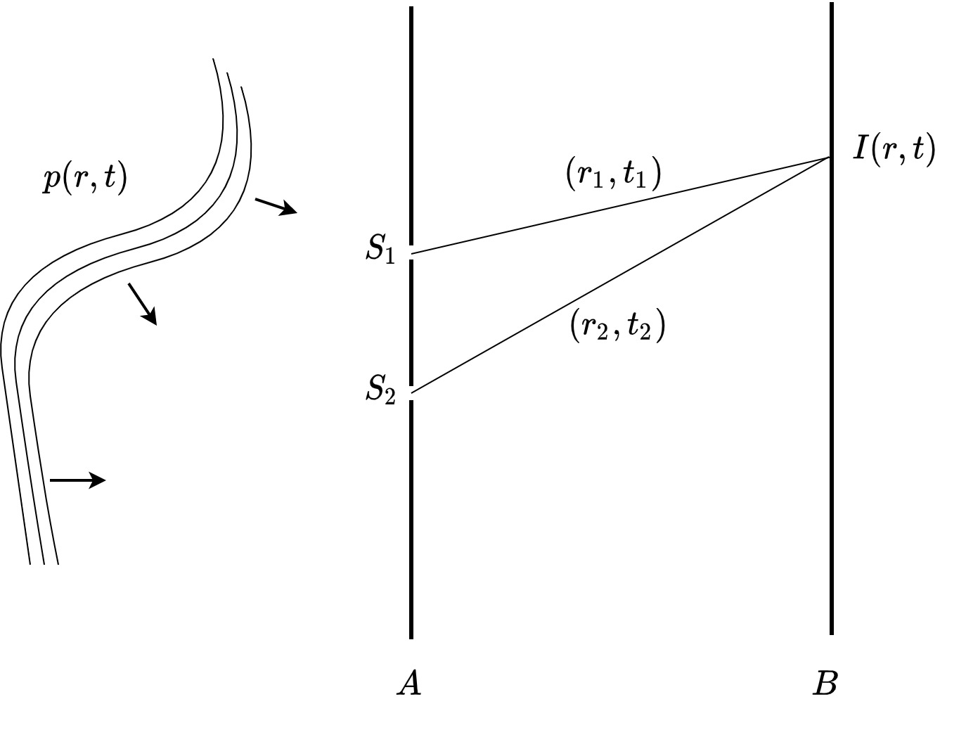
Figure 8.1: The basic setup of the coherence problem. The pressure field \(p(r,t)\) is represented by the wavefront arriving from the left that impinges on two pinholes on plane \(A\). The radiated field from the pinholes is modeled as secondary point sources, neglecting any effects of diffraction from the finite pinhole size. The sources interfere on a screen \(B\), where the intensity \(I(\boldsymbol{\mathbf{r}},t)\) is recorded.

For a pressure wave propagating from \(\boldsymbol{\mathbf{r_1}}\) and \(\boldsymbol{\mathbf{r_2}}\) to \(\boldsymbol{\mathbf{r}}\), the associated propagation time delays to the screen are

\[ t_1 = \frac{|\boldsymbol{\mathbf{r}}-\boldsymbol{\mathbf{r_1}}|}{c} \,\,\,\,\,\,\,\,\,\,\, t_2 = \frac{|\boldsymbol{\mathbf{r}}-\boldsymbol{\mathbf{r_2}}|}{c} \]

(8.4)

where \(c\) is the speed of sound in the medium. For a small source (or pinhole) size, the pressure amplitude in \(\boldsymbol{\mathbf{r}}\) is inversely proportional to the distance. We can introduce complex amplitudes \(a_1\) and \(a_2\) to designate the respective complex amplitudes in \(\boldsymbol{\mathbf{r}}\), which include also the effect of the distance. The intensity in \(\boldsymbol{\mathbf{r}}\) is therefore the ensemble average of the superposition of the pressure contributions arriving from \(\boldsymbol{\mathbf{r_1}}\) and \(\boldsymbol{\mathbf{r_2}}\), according to Eq. 8.1

\[ I(\boldsymbol{\mathbf{r}}) = |a_1|^2\langle p^*(\boldsymbol{\mathbf{r_1}},t-t_1)p(\boldsymbol{\mathbf{r_1}},t-t_1)\rangle_t + |a_2|^2\langle p^*(\boldsymbol{\mathbf{r_2}},t-t_2)p(\boldsymbol{\mathbf{r_2}},t-t_2)\rangle_t + \\ 2\Re \left[ a_1^*a_2\langle p^*(\boldsymbol{\mathbf{r_1}},t-t_1)p(\boldsymbol{\mathbf{r_2}},t-t_2)\rangle_t \right] \]

(8.5)

Using the stationarity property again, we define the mutual coherence function from the last term of Eq. 8.5

\[ \Gamma(\boldsymbol{\mathbf{r_1}},\boldsymbol{\mathbf{r_2}},\tau) = \langle p^*(\boldsymbol{\mathbf{r_1}},t)p(\boldsymbol{\mathbf{r_2}},t + \tau)\rangle_t \]

(8.6)

with a time difference variable \(\tau = t_1-t_2\), which can be measured from any time \(t\) because of stationarity. Specifically, at \(\tau=0\), the mutual coherence function \(\Gamma{\boldsymbol{\mathbf{r_1}},\boldsymbol{\mathbf{r_2}},0}\) is referred to as the mutual intensity. This is the cross-correlation function of the two pressure functions. Additionally, the average intensities right at the two pinholes are given by

\[ I_1(\boldsymbol{\mathbf{r}}) = |a_1|^2\langle p^*(\boldsymbol{\mathbf{r_1}},t)p(\boldsymbol{\mathbf{r_1}},t)\rangle_t \,\,\,\,\,\,\,\,\,\,\, I_2(\boldsymbol{\mathbf{r}}) = |a_2|^2\langle p^*(\boldsymbol{\mathbf{r_2}},t)p(\boldsymbol{\mathbf{r_2}},t)\rangle_t \]

(8.7)

where it is implied that they are shifted to \(t_1=t_2=0\) due to stationarity. Therefore, Eq. 8.5 can be rewritten as

\[ I(\boldsymbol{\mathbf{r}}) = I_1(\boldsymbol{\mathbf{r}}) + I_2(\boldsymbol{\mathbf{r}}) + 2\Re\left[ |a_1| |a_2| \Gamma(\boldsymbol{\mathbf{r_1}},\boldsymbol{\mathbf{r_2}},\tau) \right] \]

(8.8)

The first two terms represent the intensity contribution of each pinhole when the other one is blocked. We can now define the complex degree of coherence

\[ \gamma(\boldsymbol{\mathbf{r_1}},\boldsymbol{\mathbf{r_2}},\tau) = \frac{\Gamma(\boldsymbol{\mathbf{r_1}},\boldsymbol{\mathbf{r_2}},\tau)}{\sqrt{I_1(\boldsymbol{\mathbf{r}})}\sqrt{I_2(\boldsymbol{\mathbf{r}})}} = \frac{\Gamma(\boldsymbol{\mathbf{r_1}},\boldsymbol{\mathbf{r_2}},\tau)}{\sqrt{\Gamma(\boldsymbol{\mathbf{r_1}},\boldsymbol{\mathbf{r_1}},0)}\sqrt{\Gamma(\boldsymbol{\mathbf{r_2}},\boldsymbol{\mathbf{r_2}},0)}} \]

(8.9)

whose absolute value is bounded between 0 and 1 because of the normalization. We will often refer in the text to the complex degree of coherence simply as “coherence”. Using all of these, we can write the law of interference for stationary pressure fields (of plane waves), which is naturally identical to the one for scalar optical fields,

\[ I(\boldsymbol{\mathbf{r}},\tau) = I_1(\boldsymbol{\mathbf{r}}) + I_2(\boldsymbol{\mathbf{r}}) + 2\Re \left[ \sqrt{I_1(\boldsymbol{\mathbf{r}})} \sqrt{I_2(\boldsymbol{\mathbf{r}})} \gamma(\boldsymbol{\mathbf{r_1}},\boldsymbol{\mathbf{r_2}},\tau) \right] \]

(8.10)

In the narrowband approximation, the pressure wave is monochromatic and \(\gamma\) can be meaningfully expressed using a complex envelope and the following identity instead

\[ \gamma(\boldsymbol{\mathbf{r_1}},\boldsymbol{\mathbf{r_2}},\tau) \equiv |\gamma(\boldsymbol{\mathbf{r_1}},\boldsymbol{\mathbf{r_2}},\tau)| e^{i\left[ \alpha(\boldsymbol{\mathbf{r_1}},\boldsymbol{\mathbf{r_2}},\tau) -\overline{\omega} t \right]} \]

(8.11)

with \(\overline{\omega}\) being the average angular frequency and

\[ \alpha(\boldsymbol{\mathbf{r_1}},\boldsymbol{\mathbf{r_2}},\tau) = \overline{\omega} \tau + \arg \gamma(\boldsymbol{\mathbf{r_1}},\boldsymbol{\mathbf{r_2}},\tau) \]

(8.12)

The angle \(\alpha\) changes very slowly relatively to the period of the mean frequency, \(1/\overline{\omega}\). We define

\[ \delta = \overline{\omega} \tau = \overline{\omega} (t_1 - t_2) = \frac{2\pi}{\overline{\lambda}}(|\boldsymbol{\mathbf{r_1}} - \boldsymbol{\mathbf{r_2}}|) \]

(8.13)

where \(\overline{\lambda} = 2\pi c/\overline{\omega} \) is the mean wavelength. Thus, the interference law of Eq. 8.10 can be rewritten

\[ I(\boldsymbol{\mathbf{r}},\tau) = I_1(\boldsymbol{\mathbf{r}}) + I_2(\boldsymbol{\mathbf{r}}) + 2\sqrt{I_1(\boldsymbol{\mathbf{r}})} \sqrt{I_2(\boldsymbol{\mathbf{r}})} |\gamma(\boldsymbol{\mathbf{r_1}},\boldsymbol{\mathbf{r_2}},\tau)| \cos\left[ \alpha(\boldsymbol{\mathbf{r_1}},\boldsymbol{\mathbf{r_2}},\tau) - \delta \right] \]

(8.14)

In case that the two pressure source contributions at \(\boldsymbol{\mathbf{r}}\) have equal levels, \(I = I_1(\boldsymbol{\mathbf{r}}) = I_2(\boldsymbol{\mathbf{r}})\), then Eq. 8.14 simplifies to

\[ I(\boldsymbol{\mathbf{r}},\tau) = 2I\left\{ 1 + |\gamma(\boldsymbol{\mathbf{r_1}},\boldsymbol{\mathbf{r_2}},\tau)| \cos\left[ \alpha(\boldsymbol{\mathbf{r_1}},\boldsymbol{\mathbf{r_2}},\tau) - \delta \right] \right\} \]

(8.15)

which describes the intensity fringes that form as a result of interference (for example, see Figures §7.1 and §7.2). When \(|\gamma| = 1\), the two waves are said to be completely coherent and the fringes exhibit maximum contrast with areas of no light between the peaks. When \(|\gamma| = 0\), no interference takes place and the two waves are completely incoherent, yielding a constant intensity pattern with no fringes. Everything in between, \(0 < |\gamma| < 1\), is partially coherent, which entails reduced fringe contrast with decreasing degree of coherence, until they are no longer visible (see Figure 8.2). It is possible to quantify the fringe contrast using the maximum and minimum intensities obtained when the cosine is maximum

\[ I_{max}(\boldsymbol{\mathbf{r}}) = 2I(1 + |\gamma(\boldsymbol{\mathbf{r_1}},\boldsymbol{\mathbf{r_2}},\tau)|) \]

(8.16)

and minimum

\[ I_{min}(\boldsymbol{\mathbf{r}}) = 2I(1 - |\gamma(\boldsymbol{\mathbf{r_1}},\boldsymbol{\mathbf{r_2}},\tau)|) \]

(8.17)

Accordingly, the visibility of the interference pattern is defined as

\[ V = \frac{I_{max}(\boldsymbol{\mathbf{r}})-I_{min}(\boldsymbol{\mathbf{r}})}{I_{max}(\boldsymbol{\mathbf{r}}) + I_{min}(\boldsymbol{\mathbf{r}})} \]

(8.18)

which is \(V = |\gamma(\boldsymbol{\mathbf{r_1}},\boldsymbol{\mathbf{r_2}},\tau)|\) when \(I = I_1(\boldsymbol{\mathbf{r}}) = I_2(\boldsymbol{\mathbf{r}})\). In this view, the argument of \(\gamma\) determines the relative positioning of the fringes⁷⁴. For arbitrary intensities, \(I_1(\boldsymbol{\mathbf{r}}) \neq I_2(\boldsymbol{\mathbf{r}})\), the visibility can be computed in general from Eqs. 8.15 and §7.1,

\[ V = \frac{2}{\sqrt{\frac{I_1(\boldsymbol{\mathbf{r}})}{I_2(\boldsymbol{\mathbf{r}})}} + \sqrt{\frac{I_2(\boldsymbol{\mathbf{r}})}{I_1(\boldsymbol{\mathbf{r}})}}} |\gamma(\boldsymbol{\mathbf{r_1}},\boldsymbol{\mathbf{r_2}},\tau)| \]

(8.19)

The interference law of Eq. 8.14 can be rewritten in yet another way, which provides additional insight into partial coherence,

\[ I(\boldsymbol{\mathbf{r}},\tau) = |\gamma(\boldsymbol{\mathbf{r_1}},\boldsymbol{\mathbf{r_2}},\tau)| \left\{I_1(\boldsymbol{\mathbf{r}}) + I_2(\boldsymbol{\mathbf{r}}) + 2\sqrt{I_1(\boldsymbol{\mathbf{r}})} \sqrt{I_2(\boldsymbol{\mathbf{r}})} \cos\left[ \alpha(\boldsymbol{\mathbf{r_1}},\boldsymbol{\mathbf{r_2}},\tau) - \delta \right] \right\}\\ + \left[1 - |\gamma(\boldsymbol{\mathbf{r_1}},\boldsymbol{\mathbf{r_2}},\tau)|\right] \left[ I_1(\boldsymbol{\mathbf{r}}) + I_2(\boldsymbol{\mathbf{r}}) \right] \]

(8.20)

This formulation splits the interference pattern to a coherent part with intensities proportional to \(|\gamma(\boldsymbol{\mathbf{r_1}},\boldsymbol{\mathbf{r_2}},\tau)|\) and relative phase difference of \(\alpha(\boldsymbol{\mathbf{r_1}},\boldsymbol{\mathbf{r_2}},\tau) - \delta \), and an incoherent part with intensities proportional to \(1 - |\gamma(\boldsymbol{\mathbf{r_1}},\boldsymbol{\mathbf{r_2}},\tau)|\). Thus the total intensity \(I_{tot}\) is a sum of coherent and incoherent contributions, \(I_{coh}\) and \(I_{incoh}\), respectively

\[ I_{tot} = I_{coh} + I_{incoh} \]

(8.21)

Following Eq. 8.20 and neglecting the cosine term

\[ \frac{I_{coh}}{I_{incoh}} = \frac{|\gamma(\boldsymbol{\mathbf{r_1}},\boldsymbol{\mathbf{r_2}},\tau)|}{1-|\gamma(\boldsymbol{\mathbf{r_1}},\boldsymbol{\mathbf{r_2}},\tau)|} \]

(8.22)

and therefore

\[ \frac{I_{coh}}{I_{tot}} = |\gamma(\boldsymbol{\mathbf{r_1}},\boldsymbol{\mathbf{r_2}},\tau)| \]

(8.23)

This insightful formulation indicates that any partially coherent intensity pattern can be decomposed into completely coherent and completely incoherent intensity contributions.

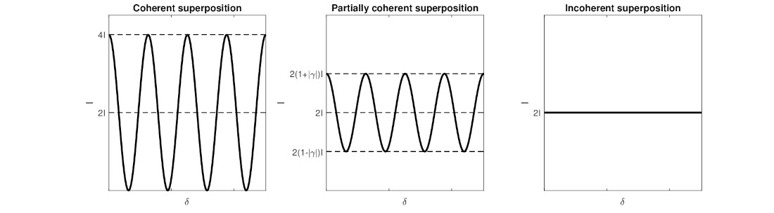
Figure 8.2: Three kinds of coherence in the simple interference experiment. The plot on the left describes complete coherence, which shows constructive interference using a coherent sum (linear in amplitude). The plot on the right shows an incoherent sum (linear in intensity) that exhibits no interference. The middle plot describes the general situation in which interference exists, but is not complete, giving rise to partial coherence. The curves can represent the visibility pattern of the fringes in an interference experiment. The plots are a reproduction of Figure 3.2 from Wolf (2007, p. 35).

Examples of coherent, partially coherent, and incoherent illuminations are given in Figure 8.3. The partially coherent objects are obtained by combining a coherent source and an incoherent source in different amounts, according to Eq. 8.21.

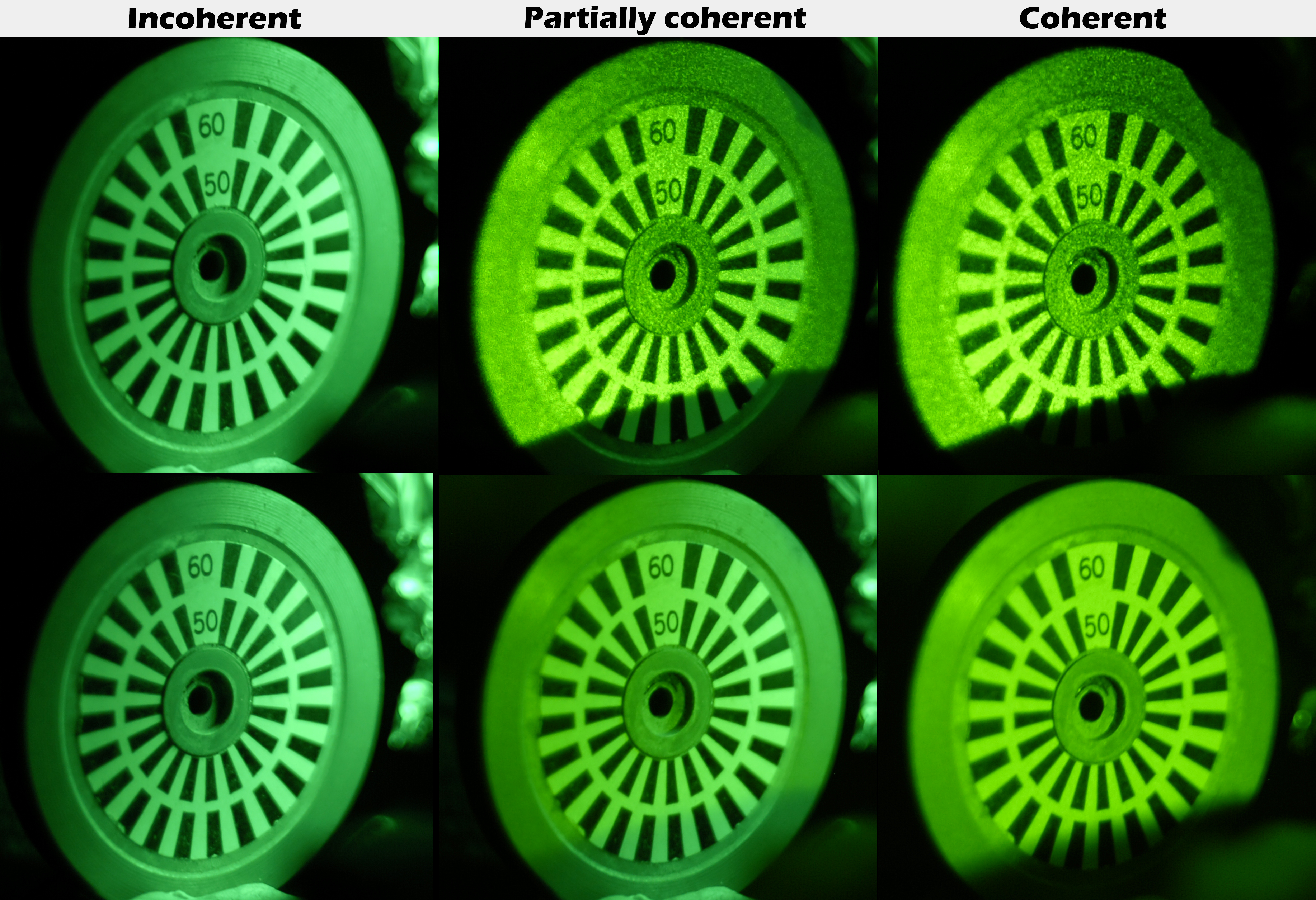
Figure 8.3: Two sets of images done under incoherent (left), partially coherent (middle), and coherent (right) illumination. The images were obtained using two different light sources. The coherent source was a green Nd:YAG laser (\(\lambda = 532\) nm), whose beam was spread with a diverging lens and a one (top) or two (bottom) different types of diffusers. The incoherent images employed a green light-emitting diode (LED) light, embedded in a bulb, of a slightly different wavelength than the laser, which is almost completely incoherent and diffuse from the source (see, for example, Mehta et al., 2010). The two light sources were illuminating the object simultaneously in the partially coherent image. However, as the laser light was significantly more intense than the LED, it was employed with different amounts of diffusion, to get different degrees of partial coherence, according to Eq. 8.21. Note that the two light sources arrive from different angles: the coherent source was almost frontal, whereas the incoherent source came from the top right of the object.

8.2.2 Temporal coherence and spatial coherence

Two idealized types of coherence are distinguished based on the expressions above. The first one is spatial coherence, \(\gamma(\boldsymbol{\mathbf{r_1}},\boldsymbol{\mathbf{r_2}},\tau_0)\), which is estimated at two different points in space, but employs a fixed time difference \(\tau_0\), usually \(\tau_0 = 0\), for convenience. The second type is temporal coherence, \(\gamma(\boldsymbol{\mathbf{r}},\boldsymbol{\mathbf{r}},\tau)\), which is determined solely by the time difference \(\tau\) assuming that the measurement positions of the two disturbances are the same, \(\boldsymbol{\mathbf{r_1}} = \boldsymbol{\mathbf{r_2}}\). In real fields, the temporal and spatial coherence are not necessarily independent. Cartoon illustrations of temporal and spatial coherence are given in Figure §7.3.

For stationary acoustic signals, the temporal coherence is, in fact, the normalized autocorrelation function of \(p(\tau)\)

\[ \gamma(\boldsymbol{\mathbf{r_1}},\boldsymbol{\mathbf{r_2}},\tau) = \gamma(\boldsymbol{\mathbf{r}},\tau) = \frac{\Gamma(\boldsymbol{\mathbf{r}},\tau)}{I(\boldsymbol{\mathbf{r}})} = \frac{\int_{-\infty}^\infty p^*(\boldsymbol{\mathbf{r}},t)p(\boldsymbol{\mathbf{r}},t+\tau)dt}{\int_{-\infty}^\infty p^*(\boldsymbol{\mathbf{r}},t)p(\boldsymbol{\mathbf{r}},t) dt} = R_{pp}(\boldsymbol{\mathbf{r}}) \]

(8.24)

using Eq. 8.9. The notation \(R_{pp}\) is standard for autocorrelation in signal processing, but will not be used here.

The distinction between temporal and spatial coherence provides an informative tool for analysis on different levels. It is also regularly employed in acoustics and hearing, only not by this name. For example, one may think of interaural acoustic cross-correlation (IACC) as a spatial coherence function for the two fixed locations of the left and right ears (§8.5). Temporal coherence, in contrast, is used in some models that probe monaural hearing, which is sensitive to the time course of signals and specifically to periodicity, which appears as peaks in the autocorrelation function. However, the input in these models is often broadband, which violates the narrowband assumption and therefore behaves somewhat differently.

8.2.3 The cross-spectral density and spectrum

According to the Wiener-Khintchin theorem, the power spectral density of a wide-sense stationary random process with zero mean is the Fourier transform of its autocorrelation function. In our case, it can be applied to the mutual coherence function, so

\[ S(\boldsymbol{\mathbf{r}},\omega) = \int_{-\infty}^\infty \Gamma(\boldsymbol{\mathbf{r}},\tau) e^{-i\omega \tau} d\tau \]

(8.25)

with \(S\) being the power spectral density of the process. The inverse transform applies as well

\[ \Gamma(\boldsymbol{\mathbf{r}},\tau) = \frac{1}{2\pi}\int_{0}^\infty S(\boldsymbol{\mathbf{r}},\omega) e^{i\omega \tau} d\omega \]

(8.26)

Only positive frequencies are used in the integral with the assumption that the signal is taken to be analytic (see §6.2).

Similarly, according to the generalized Wiener-Khintchin theorem, the mutual coherence function itself—a cross-correlation function—is the Fourier transform pair of the cross-spectral density \(W\)

\[ W(\boldsymbol{\mathbf{r_1}},\boldsymbol{\mathbf{r_2}},\omega) = \int_{-\infty}^\infty \Gamma(\boldsymbol{\mathbf{r_1}},\boldsymbol{\mathbf{r_2}},\tau) e^{-i\omega \tau} d\tau \]

(8.27)

and the inverse applies again,

\[ \Gamma(\boldsymbol{\mathbf{r_1}},\boldsymbol{\mathbf{r_2}},\tau) = \frac{1}{2\pi}\int_{0}^\infty W(\boldsymbol{\mathbf{r_1}},\boldsymbol{\mathbf{r_2}},\omega) e^{i\omega \tau} d\omega \]

(8.28)

It is important to emphasize that the cross-spectral density function spectrally depends on \(\omega\) alone only in the case of stationary signals, but it is not true in the more general case of nonstationary signals that are broadband. It can be seen by inspecting the correlation function of the pressure field in spectral-spatial coordinates, assuming that the pressure function has a Fourier transform (Mandel and Wolf, 1976)

\[ \langle P^*(\boldsymbol{\mathbf{r_1}}, \omega_1) P(\boldsymbol{\mathbf{r_2}}, \omega_2) \rangle_t = \int_{-\infty} ^\infty\int^\infty_{-\infty} \langle p^*(\boldsymbol{\mathbf{r_1}}, t_1) p(\boldsymbol{\mathbf{r_2}}, t_2) \rangle_t e^{i\omega_1 t_1}e^{-i\omega_2 t_2}dt_1 dt_2 \\ = \int_{-\infty} ^\infty\int^\infty_{-\infty} \langle p^*(\boldsymbol{\mathbf{r_1}}, t_1) p(\boldsymbol{\mathbf{r_2}}, t_1+\tau) \rangle_t e^{i(\omega_1-\omega_2) t_1}e^{-i\omega_2 \tau}dt_1 d\tau \]

(8.29)

The ensemble average in the integrand is simply the mutual coherence function, which is independent of \(t_1\) for stationary signals. Therefore, the first transform gives a delta function with the frequency difference in the argument, whereas the Fourier transform of the mutual coherence is simply the cross-spectral density

\[ \langle P^*(\boldsymbol{\mathbf{r_1}}, \omega_1) P(\boldsymbol{\mathbf{r_2}}, \omega_2) \rangle_t = W(\boldsymbol{\mathbf{r_1}},\boldsymbol{\mathbf{r_2}},\omega_1) \delta(\omega_1-\omega_2) \]

(8.30)

Hence, for \(\omega_1 \neq \omega_2\), the cross-spectral density is 0, due to stationarity, which means that waves at different frequencies are completely incoherent to one another (see also Bendat and Piersol, 2011; pp. 442–448). This is not true for nonstationary processes and coherence, as will be discussed in §8.2.9.

The spectral density expressions are known in acoustics simply as “coherence”, adopted from signal processing of random processes (e.g., Shin and Hammond, 2008). They are much more commonly used in acoustics than the coherence representation (using temporal coordinates), which is sometimes referred to as (cross-)correlation and sometimes as coherence⁷⁵. A complete coherence theory using spectral coherence was derived by Wolf (1982), Wolf (1986) and will be reviewed in §8.2.6.

8.2.4 Coherence time and coherence length

It has long been known that interference effects in light cannot be empirically observed if the disturbances are too far from the (secondary) source (e.g., obtaining visible interference fringes with sunlight is limited to very short distances from the pinholes; Verdet, 1869; pp. 72–124). This is true for sound waves too—when the pressure disturbances propagate they gradually acquire phase distortion, which eventually makes them too dissimilar to be capable of interfering. It manifests as spectral broadening of the original source output, and misalignment of the phases in the superposed field functions. Two quantities are particularly handy in quantifying the reach of coherence, inasmuch as interference effects can be measured (i.e., the fringes are visible, or \(V>0\) in Eq. §7.1). The first one is coherence time, which is the relative delay that can be applied in the autocorrelation function before the fringes of the interference pattern disappear, so it can be considered effectively incoherent. The coherence time \(\Delta\tau\) is inversely proportional to the spectral bandwidth of the source \(\Delta \omega\), so that

\[ \Delta\tau \sim \frac{2\pi}{\Delta \omega} \]

(8.31)

There are different ways to prove this expression, such as by considering an ideal detector with finite integration time that would measure a different level if the input interferes with itself during integration (Born et al., 2003; pp. 352–359). A more rigorous way to define the coherence time is based on the self-coherence of the source

\[ \Gamma(\tau) = \langle p^*(\boldsymbol{\mathbf{r}},t) p(\boldsymbol{\mathbf{r}},t+\tau) \rangle_t \]

(8.32)

which is essentially its autocorrelation function. The coherence time can then be defined using the second moment of the squared modulus of the self-coherence function (the first moment is zero due to stationarity) (Mandel and Wolf, 1995; pp. 176–177)

\[ \Delta\tau^2 = \frac{\int_{-\infty}^\infty \tau^2 |\Gamma(\tau)|^2 d\tau}{\int_{-\infty}^\infty |\Gamma(\tau)|^2 d\tau } \]

(8.33)

Similarly, the effective spectral width of the source can be defined as the second moment of the spectral density function, centered around the mean frequency \(\bar{\omega}\)

\[ \Delta \omega^2 = \frac{\int_{0}^\infty (\omega-\bar{\omega})^2 S(\omega)^2 d\omega}{\int_{0}^\infty S(\omega)^2 d\omega } \]

(8.34)

where the mean frequency is the first moment

\[ \bar{\omega} = \frac{\int_{0}^\infty \omega S(\omega)^2 d\omega}{\int_{0}^\infty S(\omega)^2 d\omega } \]

(8.35)

which, for narrowband modulated sources, we normally equate with the carrier \(\bar{\omega} = \omega_c\). With some effort, it may be shown that \(\Delta \tau\) and \(\Delta \omega\) are related by the inequality (Mandel and Wolf, 1995; pp. 176–180)

\[ \Delta \tau \Delta \omega \geq \frac{1}{2} \]

(8.36)

This expression is reminiscent of the uncertainty principle for time signals and their frequency representation. The similarity is perhaps unsurprising, given the Fourier-transform pair that the autocorrelation and the spectral density form (although in this case it was established for wide-sense stationary random processes according to the Wiener-Khintchin theorem, unlike regular time signals). Just as for time signals, the inequality 8.36 becomes an equality only for a Gaussian source distribution—both its spectrum and its autocorrelation (Gabor, 1946; Goodman, 2015; pp. 158–162).

Even with the new definition of the coherence time of Eq. 8.33, it is somewhat arbitrary and may be used primarily as an approximate measure. In reality, the visibility may oscillate around \(\Delta \tau\), depending on the exact distribution of the spectrum around the mean frequency. Furthermore, obtaining a meaningful interpretation of the coherence time when the source is not monochromatic or narrowband is not straightforward, as both spectrum and self-coherence functions have multiple peaks. This is the case in most realistic acoustic sources, which requires more ad-hoc estimates, as is demonstrated in §A.

Given a finite coherence time for the source, it is also possible to define a corresponding coherence length \(\Delta l\)

\[ \Delta l = c \Delta\tau \sim \frac{2\pi c}{\Delta \omega} \]

(8.37)

The coherence length is more intuitive in spatial coherence propagation problems and may therefore be handier in binaural hearing. In contrast, the coherence time is more immediately relevant in monaural listening, as will be explored below and throughout this work.

It will be useful to refer to the coherence time (or length) as a figure of merit for the degree of coherence of a source or a signal. So a signal with relatively high coherence time and length has a high degree of coherence and vice versa.

8.2.5 The wave equation for the coherence functions

A profound property of the mutual coherence function is that it satisfies the wave equation (Wolf, 1955). This can be established relatively easily. Starting from the scalar wave equation for the pressure field

\[ \nabla^2 p(\boldsymbol{\mathbf{r}},t)= \frac{1}{c^2}\frac{\partial^2p(\boldsymbol{\mathbf{r}},t)}{\partial t^2} \]

(8.38)

We can take the complex conjugate of \(p\) on both sides of the equation, switch to a local coordinate system with \(\boldsymbol{\mathbf{r_1}}\) and \(t_1\), and multiply both sides of the equation by \(p(\boldsymbol{\mathbf{r_2}},t_2)\)

\[ \nabla_1^2 p^*(\boldsymbol{\mathbf{r_1}},t_1) p(\boldsymbol{\mathbf{r_2}},t_2)= \frac{1}{c^2}\frac{\partial^2p^*(\boldsymbol{\mathbf{r_1}},t_1)}{\partial t_1^2}p(\boldsymbol{\mathbf{r_2}},t_2) \]

(8.39)

where \(\nabla_1\) is the Laplacian in local coordinates. Now if we take the ensemble average of both sides and interchange the order of integration and differentiation

\[ \nabla_1^2 \langle p^*(\boldsymbol{\mathbf{r_1}},t_1) p(\boldsymbol{\mathbf{r_2}},t_2) \rangle_t= \frac{1}{c^2}\frac{\partial^2}{\partial t_1^2}\langle p^*(\boldsymbol{\mathbf{r_1}},t_1)p(\boldsymbol{\mathbf{r_2}},t_2) \rangle_t \]

(8.40)

Applying the wide-sense stationarity property, we can use the fact that \(\tau = t_1-t_2\) and \(\partial^2/\partial t_1^2 = \partial^2/\partial \tau^2\) and replace the ensemble average with the mutual coherence function

\[ \nabla_1^2 \Gamma(\boldsymbol{\mathbf{r_1}},\boldsymbol{\mathbf{r_2}},\tau) = \frac{1}{c^2}\frac{\partial^2 \Gamma(\boldsymbol{\mathbf{r_1}},\boldsymbol{\mathbf{r_2}},\tau)}{\partial \tau^2} \]

(8.41)

Similarly,

\[ \nabla_2^2 \Gamma(\boldsymbol{\mathbf{r_1}},\boldsymbol{\mathbf{r_2}},\tau) = \frac{1}{c^2}\frac{\partial^2 \Gamma(\boldsymbol{\mathbf{r_1}},\boldsymbol{\mathbf{r_2}},\tau)}{\partial \tau^2} \]

(8.42)

Therefore, the homogenous wave equation is satisfied for \(\Gamma(\boldsymbol{\mathbf{r_1}},\boldsymbol{\mathbf{r_2}},\tau)\), which indicates that the coherence function, while being an average quantity, propagates in space deterministically and is an inherent property of the scalar pressure field. Coherence propagation according to the wave equation is derived for different types of fields, including inhomogeneous ones with a primary radiating source (Mandel and Wolf, 1995; pp. 181–196). To the best knowledge of the author, the above equations have not been discussed with respect to acoustic fields, except in specific underwater acoustic problems (McCoy and Beran, 1976; Berman and McCoy, 1986).

Finally, it is possible to Fourier-transform both sides of Eqs. 8.41 and 8.42 using the Wiener-Khintchin theorem (Eq. 8.27) and obtain the corresponding Helmholtz wave equations for the cross-spectral density \(W(\boldsymbol{\mathbf{r_1}},\boldsymbol{\mathbf{r_2}},\omega)\)

\[ \nabla_1^2 W(\boldsymbol{\mathbf{r_1}},\boldsymbol{\mathbf{r_2}},\omega) + k^2 W(\boldsymbol{\mathbf{r_1}},\boldsymbol{\mathbf{r_2}},\omega) = 0 \]

(8.43)

\[ \nabla_2^2 W(\boldsymbol{\mathbf{r_1}},\boldsymbol{\mathbf{r_2}},\omega) + k^2 W(\boldsymbol{\mathbf{r_1}},\boldsymbol{\mathbf{r_2}},\omega) = 0 \]

(8.44)

where we changed the order of differentiation and Fourier-transform integration in the two equations and used the wavenumber definition \(k = \omega/c\).

8.2.6 Spectral coherence

A relatively late development in optical coherence theory has been the introduction of a rigorous derivation of coherence in the spatial-spectral domain (Wolf, 1982; Wolf, 1986). It bridges the gap with the coherence functions used in signal processing and acoustics. One important insight that this theory is able to provide is in accounting for the effect of passive narrowband filters on coherence. Importantly, this theory is the basis for what appears to be the most rigorous extension to date of optical coherence theory to nonstationary processes (Lajunen et al., 2005), which is most relevant to acoustics and hearing. Dispersive propagation also requires nonstationary coherence theory (Lancis et al., 2005), as does non-periodic frequency modulation in general.

The following is a non-rigorous sketch of the main steps of derivation of the spectral coherence expressions, primarily based on Wolf (2007, pp. 60–69). The initial steps are particularly technical, but they lead to familiar and intuitive results. The full derivation is found in Wolf (1982), Wolf (1986) and Mandel and Wolf (1995, pp. 213–223), which is more rigorously approached than an initial derivation of the theory that appeared in Mandel and Wolf (1976). An alternative way of derive spectral coherence was outlined by Bastiaans (1977), but is not reviewed here.

The main obstacle in formulating a spectral-coherence theory in the first place is that stationary random processes do not have a valid Fourier representation of the time signal \(p(t)\)⁷⁶. Thus,

\[ P(\omega) = \int_{-\infty}^\infty p(t) e^{-i\omega t}dt \]

(8.45)

does not exist for stationary random processes, because \(p(t)\) is not integrable as it does not converge to zero when \(t \rightarrow \pm \infty\). This means that the spectrum in its ordinary definition as a function of the ensemble average of the squared modulus of the Fourier transform of \(p(t)\) does not formally exist either. The solution to this problem harnesses the existence of a more general definition of the spectrum found in generalized harmonic analysis (Wiener, 1930), which is based on the autocorrelation function of \(p(t)\). In order to apply it, Wolf (1982) used very general assumptions about the source field—that \(\Gamma(r_1,r_2,\tau)\) is absolutely integrable with respect to \(\tau\) and that it is continuous and bounded in the domain \(\Omega\) that contains the source and the relevant points, for all \(\tau\). He showed that these assumptions can lead to certain basic conditions on the cross-spectral density that can make it suitable to be a kernel of the Fredholm integral equation⁷⁷

\[ \int_\Omega W(\boldsymbol{\mathbf{r_1}},\boldsymbol{\mathbf{r_2}},\omega)\Psi_n (\boldsymbol{\mathbf{r_1}},\omega) d^3r_1 = \lambda_n(\omega) \Psi_n (\boldsymbol{\mathbf{r_2}},\omega) \]

(8.46)

where \(W(\boldsymbol{\mathbf{r_1}},\boldsymbol{\mathbf{r_2}},\omega)\) is a matrix of the cross-spectral density, \(\Psi_n (r,\omega)\) are eigenfunctions with corresponding positive eigenvalues \(\lambda_n(\omega) \geq 0\), which are solutions to the Fredholm integral equation. A complete solution for the equation can be expressed as a sum of all the eigenfunctions that solve the equation

\[ W(\boldsymbol{\mathbf{r_1}},\boldsymbol{\mathbf{r_2}},\omega) = \sum_n \lambda_n(\omega) \Psi_n^* (\boldsymbol{\mathbf{r_1}},\omega) \Psi_n (\boldsymbol{\mathbf{r_2}},\omega) \]

(8.47)

This sum is called the coherent-mode representation of the cross-spectral density function, as each mode can be shown to be completely spatially coherent. It is a linear combination of orthonormal coherent modes at frequency \(\omega\), whose orthonormality condition is given by

\[ \int_\Omega \Psi_n^* (\boldsymbol{\mathbf{r}},\omega) \Psi_m (\boldsymbol{\mathbf{r}},\omega) d^3r = \delta_{nm} \]

(8.48)

where \(\delta_{nm}\) is the Kronecker delta that is 1 when \(n=m\) and 0 otherwise. Using this condition it can be readily shown that each individual mode \(\Psi_n\) also satisfies the wave equations 8.43 and 8.44.

Let us now continue to construct functions that can form an ensemble from which a correlation function of the cross-spectral density function can be derived. We construct a pressure-field function using the superposition of the modes \(\Psi_n\)

\[ P(\boldsymbol{\mathbf{r}},\omega) = \sum_n b_n(\omega) \Psi_n(\boldsymbol{\mathbf{r}},\omega) \]

(8.49)

where the random finite coefficients \(b_n\) are related to the eigenvalues \(\lambda_n(\omega)\) through

\[ \langle b_n^*(\omega) b_m(\omega) \rangle_\omega = \lambda_n(\omega) \delta_{nm} \]

(8.50)

Then, we can solve for the corresponding cross-correlation function

\[ \langle P^*(\boldsymbol{\mathbf{r_1}},\omega)P(\boldsymbol{\mathbf{r_2}},\omega) \rangle_\omega = \sum_n\sum_m \langle b_n^*(\omega) b_m(\omega)\rangle_\omega \Psi^*_n(\boldsymbol{\mathbf{r_1}},\omega)\Psi_m(\boldsymbol{\mathbf{r_2}},\omega) = \sum_n \lambda_n(\omega) \Psi^*_n(\boldsymbol{\mathbf{r_1}},\omega)\Psi_n(\boldsymbol{\mathbf{r_2}},\omega) \\ = W(\boldsymbol{\mathbf{r_1}},\boldsymbol{\mathbf{r_2}},\omega) \]

(8.51)

where the order of ensemble-averaging and summation was interchanged in the first equality, Eq. 8.50 was used in the second equality, and Eq. 8.47 in the last equality that established equivalence with the cross-spectral density. With these relations at hand it is now possible to derive a corresponding expression for the spectrum

\[ S(\boldsymbol{\mathbf{r}},\omega) = \langle P^*(\boldsymbol{\mathbf{r}},\omega)P(\boldsymbol{\mathbf{r}},\omega) \rangle_\omega \]

(8.52)

This formula is intuitively appealing because it has the same form of the naive interpretation of the spectrum as the squared modulus of the Fourier transform components of the field function. Instead, it is the ensemble average of its monochromatic eigenfunction representation, rather than of the direct (forbidden) Fourier transform of the stationary field.

Now, since \(P(\boldsymbol{\mathbf{r}},\omega)\) is a linear combination of the eigenfunctions \(\Psi_m (\boldsymbol{\mathbf{r}},\omega)\) (Eq. 8.49), each of which satisfies the wave equation, then \(P(\boldsymbol{\mathbf{r}},\omega)\) itself satisfies it too,

\[ \nabla^2 P(\boldsymbol{\mathbf{r}},\omega) + k^2 P(\boldsymbol{\mathbf{r}},\omega) = 0 \]

(8.53)

The interpretation of this version of the wave equation is that \(P(\boldsymbol{\mathbf{r}},\omega)\) is the spatial part of the pressure field that has a simple harmonic (monochromatic) dependence \(p(\boldsymbol{\mathbf{r}},t) = P(\boldsymbol{\mathbf{r}},\omega)e^{i\omega t}\). It emphasizes the fact that all eigenfunctions in \(P(\boldsymbol{\mathbf{r}},\omega)\) are at the same frequency and each one may be coherent in its own right. However, if the sum of \(P(\boldsymbol{\mathbf{r}},\omega)\) (Eq. 8.49) contains more than a single mode, then the ensemble may be only partially coherent.

8.2.7 Broadband interference with spectral coherence

It is now possible to derive analogous expressions for the interference setup described in §8.2.1 and Figure 8.1, but in terms of the cross-spectral density rather than intensity. The derivation follows Wolf (2007, pp. 63–66). For an alternative proof, see also Born et al. (2003, pp. 585–588).

The frequency-dependent pressure field at point \(\boldsymbol{\mathbf{r}}\) is the sum of the contributions of the pressure from points \(\boldsymbol{\mathbf{r_1}}\) and \(\boldsymbol{\mathbf{r_2}}\),

\[ P(\boldsymbol{\mathbf{r}},\omega) = a_1 P(\boldsymbol{\mathbf{r_1}},\omega)e^{ikr_1} + a_2 P(\boldsymbol{\mathbf{r_2}},\omega)e^{ikr_2} \]

(8.54)

with \(a_1\) and \(a_2\) being the complex amplitudes of the waves traveling from \(\boldsymbol{\mathbf{r_1}}\) and \(\boldsymbol{\mathbf{r_2}}\) to \(\boldsymbol{\mathbf{r}}\), respectively. Using the expression for \(S(\boldsymbol{\mathbf{r}},\omega)\) in Eq. 8.52, let us write the spectral density in \(\boldsymbol{\mathbf{r}}\)

\[ S(\boldsymbol{\mathbf{r}},\omega) = |a_1|^2 S(\boldsymbol{\mathbf{r_1}},\omega) + |a_2|^2 S(\boldsymbol{\mathbf{r_2}},\omega) + 2\Re\left[ a_1^*a_2 W(\boldsymbol{\mathbf{r_1}},\boldsymbol{\mathbf{r_2}},\omega) e^{-i\delta}\right] \]

(8.55)

where \(\delta = \omega |\boldsymbol{\mathbf{r_1}}-\boldsymbol{\mathbf{r_2}}|/\lambda\) is once again the phase associated with the path difference, \(\lambda\) is the wavelength, and the interference is now expressed by the cross-spectral density \(W(\boldsymbol{\mathbf{r_1}},\boldsymbol{\mathbf{r_2}},\omega)\). The first two terms in Eq. 8.55 are the contribution to the spectral density in \(\boldsymbol{\mathbf{r}}\) when one of the sources is switched off, so

\[ |a_1|^2 S(\boldsymbol{\mathbf{r_1}},\omega) = S_1(\boldsymbol{\mathbf{r}},\omega) \,\,\,\,\,\,\,\,\, |a_2|^2 S(\boldsymbol{\mathbf{r_2}},\omega) = S_2(\boldsymbol{\mathbf{r}},\omega) \]

(8.56)

The spectral degree of coherence \(\mu(\boldsymbol{\mathbf{r_1}},\boldsymbol{\mathbf{r_2}},\omega)\) is defined as

\[ \mu(\boldsymbol{\mathbf{r_1}},\boldsymbol{\mathbf{r_2}},\omega) = \frac{W(\boldsymbol{\mathbf{r_1}},\boldsymbol{\mathbf{r_2}},\omega)}{\sqrt{W(\boldsymbol{\mathbf{r_1}},\boldsymbol{\mathbf{r_1}},\omega) W(\boldsymbol{\mathbf{r_2}},\boldsymbol{\mathbf{r_2}},\omega)}} \\ = \frac{W(\boldsymbol{\mathbf{r_1}},\boldsymbol{\mathbf{r_2}},\omega)}{\sqrt{S(\boldsymbol{\mathbf{r_1}},\omega) S(\boldsymbol{\mathbf{r_2}},\omega)}} \]

(8.57)

We also set

\[ \mu(\boldsymbol{\mathbf{r_1}},\boldsymbol{\mathbf{r_2}},\omega) = |\mu(\boldsymbol{\mathbf{r_1}},\boldsymbol{\mathbf{r_2}},\omega)|e^{i\alpha(\boldsymbol{\mathbf{r_1}},\boldsymbol{\mathbf{r_2}},\omega)} \]

(8.58)

with \(\alpha(\boldsymbol{\mathbf{r_1}},\boldsymbol{\mathbf{r_2}},\omega) = \arg \mu(\boldsymbol{\mathbf{r_1}},\boldsymbol{\mathbf{r_2}},\omega)\). Hence, we can rewrite Eq. 8.55 as

\[ S(\boldsymbol{\mathbf{r}},\omega) = S_1(\boldsymbol{\mathbf{r}},\omega) + S_2(\boldsymbol{\mathbf{r}},\omega) + 2 \sqrt{S_1(\boldsymbol{\mathbf{r}},\omega) S_2(\boldsymbol{\mathbf{r}},\omega)} |\mu(\boldsymbol{\mathbf{r_1}},\boldsymbol{\mathbf{r_2}},\omega)| \cos\left[\alpha(\boldsymbol{\mathbf{r_1}},\boldsymbol{\mathbf{r_2}},\omega)-\delta \right] \]

(8.59)

This is the spectral interference law. Just as with the complex degree of coherence in the temporal-spatial coherence treatment earlier, it can be shown that the spectral degree of coherence \(\mu\) is bounded \(|\mu(\boldsymbol{\mathbf{r_1}},\boldsymbol{\mathbf{r_2}},\omega)| \leq 1\), where 1 indicates complete coherence, and 0 complete incoherence (Born et al., 2003; p. 911). Unlike the temporal degree of coherence, the spectral degree of coherence is defined for a single frequency component. In general, this quantity is suitable for broadband measurements and can reveal spectral effects that have relatively small intensity changes per frequency. In contrast, temporal-spatial coherence is applicable for narrowband signals, where intensity effects are visible, with few spectral effects.

Interestingly, \(\mu(\boldsymbol{\mathbf{r_1}},\boldsymbol{\mathbf{r_2}},\omega)\) is none other that the coherence function that is commonly used in acoustics and signal processing (e.g., Shin and Hammond, 2008, pp. 284–285), only backed by physical conditions that correspond to the familiar interference experiment.

When the power contributions from the two points are equal, \(S(\boldsymbol{\mathbf{r_1}},\omega) = S(\boldsymbol{\mathbf{r_2}},\omega)\), the spectral interference law simplifies to

\[ S(\boldsymbol{\mathbf{r}},\omega) = 2 S_1(\boldsymbol{\mathbf{r}},\omega) \left\{ 1 + |\mu(\boldsymbol{\mathbf{r_1}},\boldsymbol{\mathbf{r_2}},\omega)| \cos\left[\alpha(\boldsymbol{\mathbf{r_1}},\boldsymbol{\mathbf{r_2}},\omega)-\delta \right]\right\} \]

(8.60)

which assumes the form of sinusoidal modulation envelope as a function of position when two sources interfere. It also implies that, in general, the superposed spectrum of the two contributions to the field is different than the spectrum of a single one. Unlike the interference with narrowband sounds that was analyzed using temporal coherence, spectral modulation is not sensitive to the distance from the source in the same way, and fluctuations in the spectrum may be observed well beyond the coherence time and length of the source. In some conditions, this can potentially give rise to one-half of spectrotemporal modulation that has been studied with broadband acoustic stimuli (Aertsen et al., 1980b; Aertsen et al., 1980a; Aertsen and Johannesma, 1981), primarily with respect to their cortical responses (see also §2.4.3 and §3.4.4).

8.2.8 Narrowband filtering and coherence

Before leaving the realm of stationary coherence, let us also explore the effect of linear narrowband filtering on the broadband spectral coherence function (Wolf, 1983, Wolf, 2007; pp. 73–76 and Mandel and Wolf, 1995; pp. 174–176). This problem is particularly relevant in hearing, because of the cochlear bandpass filtering property—albeit nonlinear in its transient response—which affects the received coherence of the auditory signal.

The output cross-spectral density function \(W_o\) of the input pressure field \(P\), which passes through a bandpass filter that has a transfer function \(H(\omega)\), is

\[ W_o(\boldsymbol{\mathbf{r_1}},\boldsymbol{\mathbf{r_2}},\omega) = \langle H^*(\omega)P^*(\boldsymbol{\mathbf{r_1}},\omega) H(\omega)P(\boldsymbol{\mathbf{r_2}},\omega) \rangle_\omega = |H(\omega)|^2 \langle P^*(\boldsymbol{\mathbf{r_1}},\omega) P(\boldsymbol{\mathbf{r_2}},\omega) \rangle_t \\ = |H(\omega)|^2 W_i(\boldsymbol{\mathbf{r_1}},\boldsymbol{\mathbf{r_2}},\omega) \]

(8.61)

where \(W_i\) is the cross-spectral density function before the filter, at the input. In the second equality, \(H(\omega)\) was taken out of the ensemble average because it is deterministic. It results in the familiar input-output relation of the linear filter, with the cross-spectral density function assuming the role of the signal. It is then straightforward to show that the spectral degree of coherence is unaffected by the filter. At the input it is

\[ \mu_i(\boldsymbol{\mathbf{r_1}},\boldsymbol{\mathbf{r_2}},\omega) = \frac{W_i(\boldsymbol{\mathbf{r_1}},\boldsymbol{\mathbf{r_2}},\omega)}{\sqrt{W_i(\boldsymbol{\mathbf{r_1}},\boldsymbol{\mathbf{r_1}},\omega) W_i(\boldsymbol{\mathbf{r_2}},\boldsymbol{\mathbf{r_2}},\omega)}} \]

(8.62)

And at the output

\[ \mu_o(\boldsymbol{\mathbf{r_1}},\boldsymbol{\mathbf{r_2}},\omega) = \frac{ W_o(\boldsymbol{\mathbf{r_1}},\boldsymbol{\mathbf{r_2}},\omega)}{\sqrt{W_o(\boldsymbol{\mathbf{r_1}},\boldsymbol{\mathbf{r_1}},\omega) W_o(\boldsymbol{\mathbf{r_2}},\boldsymbol{\mathbf{r_2}},\omega)}} \\ = \frac{|H(\omega)|^2 W_i(\boldsymbol{\mathbf{r_1}},\boldsymbol{\mathbf{r_2}},\omega)}{\sqrt{|H(\omega)|^2 W_i(\boldsymbol{\mathbf{r_1}},\boldsymbol{\mathbf{r_1}},\omega) |H(\omega)|^2 W_i(\boldsymbol{\mathbf{r_2}},\boldsymbol{\mathbf{r_2}},\omega)}} = \mu_i(\boldsymbol{\mathbf{r_1}},\boldsymbol{\mathbf{r_2}},\omega) \]

(8.63)

Moving now to the spatial-temporal complex degree of coherence \(\gamma(\boldsymbol{\mathbf{r_1}},\boldsymbol{\mathbf{r_2}},\tau)\), we repeat Eq. 8.9 using the self-coherence functions in the denominator:

\[ \gamma(\boldsymbol{\mathbf{r_1}},\boldsymbol{\mathbf{r_2}},\tau) = \frac{\Gamma(\boldsymbol{\mathbf{r_1}},\boldsymbol{\mathbf{r_2}},\tau)}{\sqrt{\Gamma(\boldsymbol{\mathbf{r_2}},\boldsymbol{\mathbf{r_2}},0)}\sqrt{\Gamma(\boldsymbol{\mathbf{r_2}},\boldsymbol{\mathbf{r_2}},0)}} \]

(8.64)

We would like to find out whether \(\gamma(\boldsymbol{\mathbf{r_1}},\boldsymbol{\mathbf{r_2}},\tau)\) is affected by the filter, unlike \(\mu(\boldsymbol{\mathbf{r_1}},\boldsymbol{\mathbf{r_2}},\omega)\). It is possible to use the Wiener-Khintchin theorem and express the cross-correlations as the inverse Fourier transform of the cross-spectral density (Eq. 8.28), so at the input to the filter we get

\[ \Gamma_i(\boldsymbol{\mathbf{r_1}},\boldsymbol{\mathbf{r_2}},\tau) = \frac{1}{2\pi} \int_{0}^\infty W_i(\boldsymbol{\mathbf{r_1}},\boldsymbol{\mathbf{r_2}},\omega) e^{i\omega \tau} d\omega \]

(8.65)

whereas at the output it is

\[ \Gamma_o(\boldsymbol{\mathbf{r_1}},\boldsymbol{\mathbf{r_2}},\tau) = \frac{1}{2\pi} \int_{0}^\infty W_o(\boldsymbol{\mathbf{r_1}},\boldsymbol{\mathbf{r_2}},\omega) e^{i\omega \tau} d\omega = \frac{1}{2\pi} \int_{0}^\infty |H(\omega)|^2 W_i(\boldsymbol{\mathbf{r_1}},\boldsymbol{\mathbf{r_2}},\omega) e^{i\omega \tau} d\omega \\ \approx \frac{1}{2\pi} W_i(\boldsymbol{\mathbf{r_1}},\boldsymbol{\mathbf{r_2}},\omega_c) \int_{0}^\infty |H(\omega)|^2 e^{i\omega \tau} d\omega \]

(8.66)

where the final approximation used was done by assuming that the cross-spectral density is about constant across the narrow filter bandwidth, so it could be taken out of the integral. Generalizing across the two positions of \(\boldsymbol{\mathbf{r}}\)

\[ \Gamma_o(\boldsymbol{\mathbf{r_m}},\boldsymbol{\mathbf{r_n}},\tau) \approx \frac{1}{2\pi} W_i(\boldsymbol{\mathbf{r_m}},\boldsymbol{\mathbf{r_n}},\omega_c) \int_{0}^\infty |H(\omega)|^2 e^{i\omega \tau} d\omega \,\,\,\,\,\,\,\,\,\, m,n = 1,2 \]

(8.67)

Therefore, the complex degree of coherence is

\[ \gamma_o(\boldsymbol{\mathbf{r_1}},\boldsymbol{\mathbf{r_2}},\tau) \approx \frac{W_i(\boldsymbol{\mathbf{r_1}},\boldsymbol{\mathbf{r_2}},\omega_c) \int_{0}^\infty |H(\omega)|^2 e^{i\omega \tau} d\omega}{ \sqrt{W_1(\boldsymbol{\mathbf{r_1}},\boldsymbol{\mathbf{r_1}},\omega_c) W_2(\boldsymbol{\mathbf{r_2}},\boldsymbol{\mathbf{r_2}},\omega_c)} \int_{0}^\infty |H(\omega)|^2 d\omega } = \mu_i(\boldsymbol{\mathbf{r_1}},\boldsymbol{\mathbf{r_2}},\omega_c) \frac{\int_{0}^\infty |H(\omega)|^2 e^{i\omega \tau} d\omega}{\int_{0}^\infty |H(\omega)|^2 d\omega} \]

(8.68)

where we used Eqs. 8.64, 8.66, and 8.67. The integral of Eq. 8.68 can be simplified by inspecting the value of \(\gamma_o(\boldsymbol{\mathbf{r_1}},\boldsymbol{\mathbf{r_2}},\tau)\) around \(\tau = 0\). The quotient is the normalized Fourier transform of \(|H(\omega)|^2\)—essentially the normalized impulse response function of the filter, measured for intensity, and assuming that the filter is linear. This gives us a maximum at \(\tau = \tau_0 \geq 0\), for a causal filter, so that

\[ \gamma_o(\boldsymbol{\mathbf{r_1}},\boldsymbol{\mathbf{r_2}},\tau) \leq \gamma_o(\boldsymbol{\mathbf{r_1}},\boldsymbol{\mathbf{r_2}},\tau_0) = \mu_i(\boldsymbol{\mathbf{r_1}},\boldsymbol{\mathbf{r_2}},\omega_c) \]

(8.69)

This result mirrors the narrowband nature of the coherence function \(\gamma_o(\boldsymbol{\mathbf{r_1}},\boldsymbol{\mathbf{r_2}},\tau)\). It predicts that the temporal degree of coherence is not guaranteed to remain the same given the narrowband filtering. Even for very narrow bandwidths it may well be less than unity. But we can obtain further insight than that, by testing the effect of the bandwidth of an ideal rectangular bandpass filter on the coherence function. If we set

\[ |H_r(\omega)|^2 = 1 \,\,\,\,\,\,\,\, \omega_c - \frac{\Delta\omega}{2} \leq \omega \leq \omega_c + \frac{\Delta\omega}{2} \]

(8.70)

for a filter with bandwidth \(\Delta\omega\). Then we can directly compute Eq. 8.68, which gives

\[ \gamma_o(\boldsymbol{\mathbf{r_1}},\boldsymbol{\mathbf{r_2}},\tau) \approx \mu_i(\boldsymbol{\mathbf{r_1}},\boldsymbol{\mathbf{r_2}},\omega_c) \Delta\omega e^{i\omega_c\tau}\mathop{\mathrm{sinc}}\left( \Delta \omega \tau \right) \]

(8.71)

where \(\mu_i(\boldsymbol{\mathbf{r_1}},\boldsymbol{\mathbf{r_2}},\omega_c)\) has the dimensions of spectral density, so it cancels out the scaling by \(\Delta \omega\). The main lobe of the sinc function becomes narrower with increasing filter bandwidth. We remember that the coherence time of a narrowband source is inversely proportional to its bandwidth (Eq. 8.31). Here we showed how the narrowband filtering can effectively turn a broadband source into a narrowband one when the bandwidth is narrow enough, which results in an increase of the coherence time. This would make a broadband source appear more coherent than it is at the origin. This is an important result that we will revisit throughout this work. See also Jacobsen and Nielsen (1987) for an alternative derivation.

8.2.9 Nonstationary coherence

Coherence theory as has been formulated until recently is largely based on the theory of random stationary processes. Even though it has proven to have a tremendous explanatory power in optics and is just as applicable in other scalar wave phenomena, it is inadequate to deal with realistic acoustic signals that are, by and large, nonstationary. The importance of nonstationarity was expressed by Antoni (2009) in the context of cyclostationary acoustic signal analysis, which reveals hidden periodicities (modulations) in the standard power spectrum: “Let us insist on the assertion that nonstationarity—as evidenced by the presence of transients—is intimately related to the concept of information. This is completely analogous to speech or music signals that can carry a message or a melody only because they consist of a succession of nonstationarities.”

Formal work on nonstationary optical coherence theory started only relatively recently with Bertolotti et al. (1995). We shall adopt a similar but more rigorous theory by Lajunen et al. (2005), which is a close variation on the spectral coherence theory presented in §8.2.6. Therefore, it is not going to be necessary to consider all the steps in the derivation, but rather to discuss the main differences and implications.

Nonstationary coherence theory is defined for a pulse train, in which the pulses are well-separated in time from one another, so they do not mix. Pulses here should be seen as a very general way to express a finite wave that has a beginning and an ending, although its duration is not constrained by the analysis. The pulses can be different from one another in level, spectrum, position, and duration, which means that the ensemble is certainly not ergodic. Hence, nonstationary ensemble averages that are employed here are not time averages as before, but have to be computed on a pulse-by-pulse basis, where every pulse is defined with its own time reference—independently of the other pulses. Therefore, the expression for the mutual coherence function takes the form

\[ \Gamma(\boldsymbol{\mathbf{r_1}},\boldsymbol{\mathbf{r_2}},t_1,t_2) = \langle p^*(\boldsymbol{\mathbf{r_1}},t_1)p(\boldsymbol{\mathbf{r_2}},t_2) \rangle = \frac{1}{N}\sum_{n=1}^N p_n^*(\boldsymbol{\mathbf{r_1}},t_1)p_n(\boldsymbol{\mathbf{r_2}},t_2) \]

(8.72)

where the pressure field \(p\) of each pulse is marked with a subscript \(n\). Because of the nonstationarity of the pulse train, the cross-correlation is not time-invariant, in general, which is underscored by the ensemble averaging operation \(\langle \cdots \rangle\) not carrying the subscript \(t\) this time. The nonstationary complex degree of coherence is (Bertolotti et al., 1995)

\[ \gamma(\boldsymbol{\mathbf{r_1}},\boldsymbol{\mathbf{r_2}},t_1,t_2) = \frac{\Gamma(\boldsymbol{\mathbf{r_1}},\boldsymbol{\mathbf{r_2}},t_1,t_2)}{\sqrt{I(\boldsymbol{\mathbf{r_1}},t_1)}\sqrt{I(\boldsymbol{\mathbf{r_2}},t_2)}} \]

(8.73)

Similarly, the nonstationary cross-spectral density is

\[ W(\boldsymbol{\mathbf{r_1}},\boldsymbol{\mathbf{r_2}},\omega_1,\omega_2) = \langle P^*(\boldsymbol{\mathbf{r_1}},\omega_1)P(\boldsymbol{\mathbf{r_2}},\omega_2) \rangle = \frac{1}{N}\sum_{n=1}^N P_n^*(\boldsymbol{\mathbf{r_1}},\omega_1)P_n(\boldsymbol{\mathbf{r_2}},\omega_2) \]

(8.74)

Here the most striking feature of the nonstationary theory is revealed, as disturbances of different frequencies can interact—unlike in the stationary case where different frequencies are completely incoherent. The nonstationary spectral degree of coherence is then

\[ \mu(\boldsymbol{\mathbf{r_1}},\boldsymbol{\mathbf{r_2}},\omega_1,\omega_2) = \frac{W(\boldsymbol{\mathbf{r_1}},\boldsymbol{\mathbf{r_2}},\omega_1,\omega_2)}{\sqrt{S(\boldsymbol{\mathbf{r_1}},\omega_1)}\sqrt{S(\boldsymbol{\mathbf{r_2}},\omega_2)}} \]

(8.75)

All steps and expressions in the derivation are completely analogous to the stationary case as described in 8.2.6, but with the frequency variables differentiated \(\omega_1 \neq \omega_2\) everywhere where cross-correlation is applied. Notably, the nonstationary mutual coherence and cross-spectral density both satisfy the wave equation, just like Eqs. 8.41, 8.42, 8.43, and 8.44.

The option of using time-dependent ensemble averages instead of mutual coherence was mentioned in Mandel and Wolf (1965), where it was referred to as the ensemble correlation function. It was not further pursued there, because of the greater usefulness of stationarity. Derode and Fink (1994) suggested, independently, to use this alternative averaging in acoustical nonstationary signals, anticipating the nonstationary optical theory. However, their acoustic coherence theory did not consider frequency interaction in its spectral coherence functions. Nonstationary acoustic signal theory was also derived by Mark (1970), but without considering an interaction between frequencies either, so \(\omega_1=\omega_2\), just as in stationary processes. The coherence between of two frequencies that propagate in turbulent conditions was investigated by Havelock et al. (1998), but the analysis referred to an envelope-like fluctuation term that is common to the two frequencies and becomes gradually decohered with increasing turbulence strength and range, for fixed points in time and space. This usage is more similar to the definition of coherence in hearing science (§7.2.4).

In general, nonstationary processes are much more complicated to work with than stationary processes. As a rule, since the frequency components are not independent in nonstationary processes, it is possible that the usual self-coherence function does not fully capture its second-order statistical properties as in stationary processes (e.g., the spectrum and the coherence time). This can result in analytic signals that are not “proper”, which means that their real and imaginary parts are not independent and their cross-correlation does not cancel out as Eq. §6.14 predicts (Neeser and Massey, 1993; Picinbono, 1994). It has been suggested that realistic signals such as speech are improper, which may require different applied tools to deal with them (Picinbono and Bondon, 1997; Schreier and Scharf, 2003; Clark, 2012). It was recently suggested by Clark (2012) that phase-locked coherent tracking (using the complex envelope formalism) may go a long way to accurately demodulate improper signals (i.e., obtain accurate audio and modulation spectra), which coincides with what the ear appears to be doing, at least in part (§9). While this topic has some clear relevance to the present theory, as both deal with the borderline between constant and instantaneous quantities, this approach is outside the scope of this work.

Beating

An early example of nonstationary interference has been the demonstration of the beating between two laser sources that have nearly identical line frequencies (Magyar and Mandel, 1963). This would have not been considered a particularly interesting achievement in acoustics, but the analysis provides a useful formulation to beating using coherence theory. In this case, the ensemble average was not employed, because it would have effectively randomized the initial phase, which in the long run eliminates the contrast of any measurable beating. The spatial coordinate is assumed constant in all expressions, so it is incorporated into the phase

\[ p_1(t) = \sqrt{I_1(t)} \exp ( i\omega_1 t + i\varphi_1 ) \,\,\,\,\,\,\, p_2(t) = \sqrt{I_2(t)} \exp ( i\omega_2 t + i\varphi_2) \]

(8.76)

with the initial phase terms \(\varphi_1\) and \(\varphi_2\). In general, there is a different initial phase, as well as a possible path difference \(c\tau\) between the wavefronts that corresponds to a delay \(\tau\). We can write the interference law for the fields \(p_1(t-\tau/2)\) and \(p_2(t+\tau/2)\) using all the phase contributions

\[ I(t) = I_1(t) + I_2(t) + 2\sqrt{I_1(t)I_2(t)} \cos\left[ (\omega_2-\omega_1)t + \frac{1}{2}(\omega_2+\omega_1)\tau + \varphi_2 - \varphi_1\right] \]

(8.77)

The intensity will vary in time as long as \(\omega_1 \neq \omega_2\). This beating can be thought of as temporal fringes given that mathematically there is no difference with spatial interference except for the changed space-time coordinate. Assuming a detector that has a rectangular input window \(T\), we can integrate the intensity and obtain the detected beating

\[ \hat{I}(t,T) = \frac{1}{T}\int_t^{t+T} I(t')dt' \\ = I_1(t) + I_2(t) + 2\sqrt{I_1(t)I_2(t)} \mathop{\mathrm{sinc}} \left[\frac{(\omega_1-\omega_2)T}{2}\right] \cos\left[ (\omega_2-\omega_1)\left(t+\frac{T}{2}\right) + \frac{1}{2}(\omega_2+\omega_1)\tau + \varphi_2 - \varphi_1\right] \]

(8.78)

Based on Eq. 8.19 we obtain the visibility pattern, which is stationary in comparison with the time-dependent cosine term

\[ |\gamma(t)| = \frac{2}{ \sqrt{\frac{I_1(t)}{I_2(t)}} + \sqrt{\frac{I_2(t)}{I_1(t)}} }\mathop{\mathrm{sinc}} (\pi \Delta f T ) \]

(8.79)

for spacing between the frequencies of \(\Delta f = |f_2-f_1|\). By exchanging audibility for visibility, this equation provides a condition for beating detection. However, the rectangular integration window causes the audibility to fluctuate with the \(\Delta f\) due to the side lobes of the sinc function, which is psychoacoustically not the case. Rather, the beating audibility should diminish monotonically with \(\Delta f\). Therefore, the rectangular window may be replaced with a Gaussian window that has the same equivalent rectangular bandwidth \(T\) (see §B.3)

\[ \hat{I}(t,T) = \frac{1}{T} \int_{-\infty}^{\infty} I(t')\exp \left( -4\ln2 \,\, \frac{t^{'2}}{T^2} \right) dt' \\ = I_1(t) + I_2(t) + \sqrt{\frac{\pi}{\ln 2}}\sqrt{I_1(t)I_2(t)} \exp\left[ -\frac{(\pi T \Delta f)^2}{4\ln2 \,\,}\right] \cos\left[ \frac{1}{2}(\omega_2+\omega_1)\tau + \varphi_2 - \varphi_1\right] \]

(8.80)

with the respective visibility/audibility

\[ |\gamma(t)| = \frac{\sqrt{\frac{\pi}{\ln 2}}}{ \sqrt{\frac{I_1(t)}{I_2(t)}} + \sqrt{\frac{I_1(t)}{I_2(t)}} }\exp\left[ -\frac{(\pi T \Delta f)^2}{4\ln2 \,\,}\right] \]

(8.81)

For a given \(T\) of the detector and for \(I_1 = I_2\), the audibility with the Gaussian window will drop to half for \(\Delta f = \frac{2\ln2 \,\,}{\pi T} \approx 0.441/T\), whereas with the rectangular window, it is \(\Delta f = 0.5/T\) (the first zero of the sinc function). We shall revisit this solution in §12.5.5, once the values of the auditory \(T\) will be estimated.

The phase of the degree of coherence depends on the values of \(\varphi_1\), \(\varphi_2\) and \(\tau\), which are not necessarily controlled. It means that had we taken the ensemble average, the temporal interference pattern—the beating—may no longer be audible, as the relative position of the temporal fringes would move with the phase. Therefore, in order to measure beating, we have to look at the specific instance in time, as nonstationarity requires.

8.2.10 Discussion

The classical theory of coherence was reviewed with emphasis on the most relevant aspects to auditory processing of acoustic signals. Although many of the theoretical results have been undoubtedly known and used by acousticians, there is an obvious lack of systematic treatments or reviews of this important topic within the field. It is appreciated that some of the results are imprecise in the near-field approximation, where the sound intensity is directional and evanescent modes can be dominant. Nevertheless, the squared pressure is the most useful proxy for acoustic intensity and power in the majority of practical cases. It is also the most immediate measurement when using pressure detectors such as the ears and standard pressure microphones. This makes the classical coherence theory highly relevant for hearing research as well.

The remainder of this chapter is therefore dedicated to the exploration of how coherence theory has been applied in hearing-relevant acoustics, sometimes using different terminology than in optics. In turn, the insight garnered in these sections will provide the necessary basis for understanding the coherent-incoherent distinction that is key to the imaging auditory system.

8.3 Coherence of typical acoustic sources

8.3.1 Mathematical sounds and realistic light sources

It can be easy to forget that natural acoustic signals are not pure in the mathematical sense. In the context of coherence, the infinitesimal spectral width of the pure tone entails that, asymptotically, it has infinite coherence time and length. From the coherence time definitions (Eq. 8.31), the coherence time for a mathematical pure tone is

\[ \Delta \tau_{pure\,tone}\rightarrow \infty \]

(8.82)

whereas for white noise—the other mathematically idealized sound stimulus—it is

\[ \Delta \tau_{white\,noise} \rightarrow 0 \]

(8.83)

While somewhat trivial, these extreme cases are important because they map to many of the experiments done in both acoustic and auditory research since the advent of electronics. In the present work, these extreme coherence properties inform the interpretation of published results that were obtained using such signals. Unlike signals of finite bandwidth, broadening of pure tones (i.e., through absorption, dispersion, reflections, and the Doppler effect) accumulates very slowly, to the point of being negligible in normal settings (see Figures §3.1 and §3.2 for illustrations using dispersion). This means that effects that have to do with partial coherence may not be readily encountered in laboratory-based experiments and calculations based on pure tones.

In contrast to both pure tones and white noise, realistic optical sources have finite bandwidths, so they exhibit a broader range of coherence phenomena. Only with the invention of the laser (and maser, both in the 1950s) did experimental optics obtain stable quasi-monochromatic sources, which have much narrower spectral bandwidths than natural sources (yet still finite)⁷⁸. For example, Wolf (2007, p. 5) compared the coherence time and length of a gas discharge lamp of \(\Delta\tau \approx 0.01\,\,\mu\mathop{\mathrm{s}}\) and \(\Delta l \approx 19\) m to a stabilized laser of \(\Delta\tau \approx 100\,\,\mu\mathop{\mathrm{s}}\) and \(\Delta l \approx 190\) km(!). Note, however, that these sources still have finite bandwidths of \(\Delta f \sim 10^{8}\) Hz for the lamp and \(\Delta f \sim 10^{4}\) Hz for the laser. While the exact center frequency was not provided by Wolf, we can roughly assume it to be \( 10^{14}\) Hz in both cases, which would make the relative bandwidth of the two sources \(10^{-6}\) and \(10^{-10}\), respectively. While in optics these sources are still not considered pure tones—their phase cannot be controlled as in sound generation—equivalent precision in audio would be very impressive. For a tone at 1000 Hz, it would entail approximate precision of 0.001 Hz and 0.0000001 Hz, respectively—well below the resolution of any standard acoustic instrumentation.

In the following, we will try to understand what kind of coherence properties may be expected from realistic acoustic sources. Due to the relative scarcity of data in literature, this question can be answered only in part.

8.3.2 Effective duration of realistic acoustic sources

The coherence time of acoustic sources may be estimated directly from the autocorrelation function of the radiated output in free field (Eq. 8.33). There is relatively little information available in literature about the coherence properties of typical acoustic sources and most work has focused on (broadband) music and the interaction it has with room acoustics (e.g., Ando, 1985). As most natural acoustic sources are nonstationary, some kind of running autocorrelation is required to be able to estimate their temporal coherence. In general, these sources are not at all as well-behaved as the optical sources used in stationary coherence theory, and their coherence time can only be estimated approximately. If the stationary autocorrelation function is computed using the limit

\[ \Gamma(\tau) = \lim_{T \rightarrow \infty} \frac{1}{2T} \int_{-T}^T p^*(t)p(t+\tau)dt \]

(8.84)

Then, in the nonstationary case, the integration constant \(T\) is finite and its value affects the measurement. A longer \(T\) can be used to detect slower periodicities and features in the coherence function. Examples of the effect of the choices of \(T\) on the autocorrelation function of several musical pieces are shown in Figures 3.4–3.6 in Ando (1998, pp. 14–18) and for other sounds in Figure §A.2. These figures demonstrate how signals differ in their sensitivity to \(T\), which may or may not capture their characteristic coherence time. Therefore, \(T\) has to be selected with consideration to the degree of coherence of the sound that is being analyzed.

In several acoustic studies that estimated the running autocorrelation, a measure similar to coherence time—the effective duration (usually denoted with \(\tau_e\))—was defined as the -10 dB drop from the autocorrelation peak at \(\tau=0\) (i.e., when \(|\gamma|=0.1\)), but extrapolated from the initial 5 dB drop in the response peak. This definition produces an exaggerated effect compared to the coherence time in the optical definition that entails only a 3 dB drop from the peak (half-width maximum power). As the procedure to obtain the 10 dB point normally involves a linear fit to the autocorrelation function of the A-weighted pressure (e.g., Ando, 1998, pp. 12–13), the conversion entails that \(\Delta\tau \approx 0.3 \tau_c\), if the autocorrelation function is well-behaved. Different methods exist to estimate the running autocorrelation and the slope of its main peak, so the estimates of the effective durations of acoustic sources tend to be somewhat inconsistent between reports and should be taken only as approximate ranges (D'Orazio et al., 2011). This is also apparent from the supplementary analyses presented in §A.

While the criterion for the effective duration definition seems to have been arbitrarily set, it has been associated with some behavioral measures. Notably, identification of monosyllables by moderately hearing-impaired elderly listeners was highly correlated (\(r=0.87\)) with the effective duration of the syllables, but not with the broadband coherence time analog⁷⁹ (\(r=0.19\)) (Shimokura et al., 2017; Figure 5d–5e). In another study, Ando (1998, pp. 88–119) found several correlations between the preference of ideal reverberation time for specific music types and the effective duration of the music. A “temporal factor” was also defined that is equivalent to coherence time of the broadband autocorrelation, set at half the power of the main lobe, and was found to correlate with the timbre perception of spectral tilt of distortion guitar (Ando and Cariani, 2009; pp. 11 and 120–124).

The effective duration—and more generally, the degree of coherence—of speech signals has not been systematically surveyed in the literature, even though autocorrelation is frequently used in signal processing of speech (e.g., for extracting the instantaneous fundamental frequency; Kawahara et al., 1999 and De Cheveigné and Kawahara, 2002). While speech contains periodic or quasi-periodic components—especially in vowels (see §3.3.2)—it is highly nonstationary and dynamic, and therefore cannot be expected to have very long effective duration on average, especially when it is calculated for the broadband signal. According to D'Orazio and Garai (2017), speech has an effective duration of somewhere between 8 and 16 ms. This estimate was probably based on Ando (1998, Figure 4.2), who found a range of effective durations with an average of 12 ms (measured with a Japanese poem spoken by a female reader). That even speech vowels are not completely periodic can be seen in the autocorrelation curves in Hillenbrand (1988, Figure 2), which reveal large, but nowhere near infinite effective duration for a sustained /a/ vowel—about 10–20 pitch periods for both real and synthesized male and female voices. Converted to time units, it can correspond to a range of 50–200 ms for a male with fundamental frequency of \(f_0=100\) Hz at the low end, or to \(f_0=200\) Hz for a female voice at the high end. A more detailed study of female Japanese monosyllables found that the effective duration is 30–70 ms (Shimokura et al., 2017). An older study with no specific details about the exact signal used reported male speech to have effective duration of about 100 ms, but the autocorrelation curve never tapered off below \(|\gamma| \approx 0.15\) (Fourdouiev, 1965; Figure 2 and table). Interpolation of the same curve gives a coherence time of about 31 ms for speech.

More data has been collected about the coherence of musical sources than about speech sources. For example, Ando (1998, pp. 13–19) compared the running autocorrelation of different piano performances and found a wide range of effective durations with a minimum of 20–30 ms (e.g., Ando's Figure 3.5d), along with instances of much longer durations (\(>\) 200 ms, Figure 3.4d), depending on the integration time used in the calculation.

Effective duration data of non-musical acoustic sources have been reported sporadically. For example, autocorrelation measurements of narrowband noise centered around 250, 1000, and 4000 Hz with \(\Delta f = \) 213, 554, and 1556 Hz, respectively, found coherence time (for \(|\gamma|=0.5\)) that is scaled by the noise bandwidth of about \(\Delta \tau = \) 3, 1.5, and 0.4 ms, respectively (Ando and Alrutz, 1982), as expected from the coherence time definition. In another study, the temporal characteristics of ground-level broadband noise from a landing airplane at 1 km altitude were estimated and found to become incoherent very quickly (1–2 ms) (Fujii et al., 2001). However, there were additional peaks in the autocorrelation function after the initial drop that represent spurious coherence due to periodic components of the aircraft noise.

A qualitative breakdown of the coherence of various signal families was provided recently by D'Orazio and Garai (2017, Figures 4 and 6), in which the relative effective duration of speech, music, pure tones, which noise, impulses, ventilation sound, and “glitch” sounds were all plotted against an impulsiveness scale (ranging between completely impulsive and completely continuous). As many musical pieces contain sounds that are both continuous and periodic (e.g., harmony of a string section) as well as impulsive sounds with very slow rhythmic periods (e.g, drum beat), its effective durations occupies a large range of times (16–512 ms), depending on the musical content and instrumentation. The figure is roughly reproduced in Figure 8.4 with slight modifications.

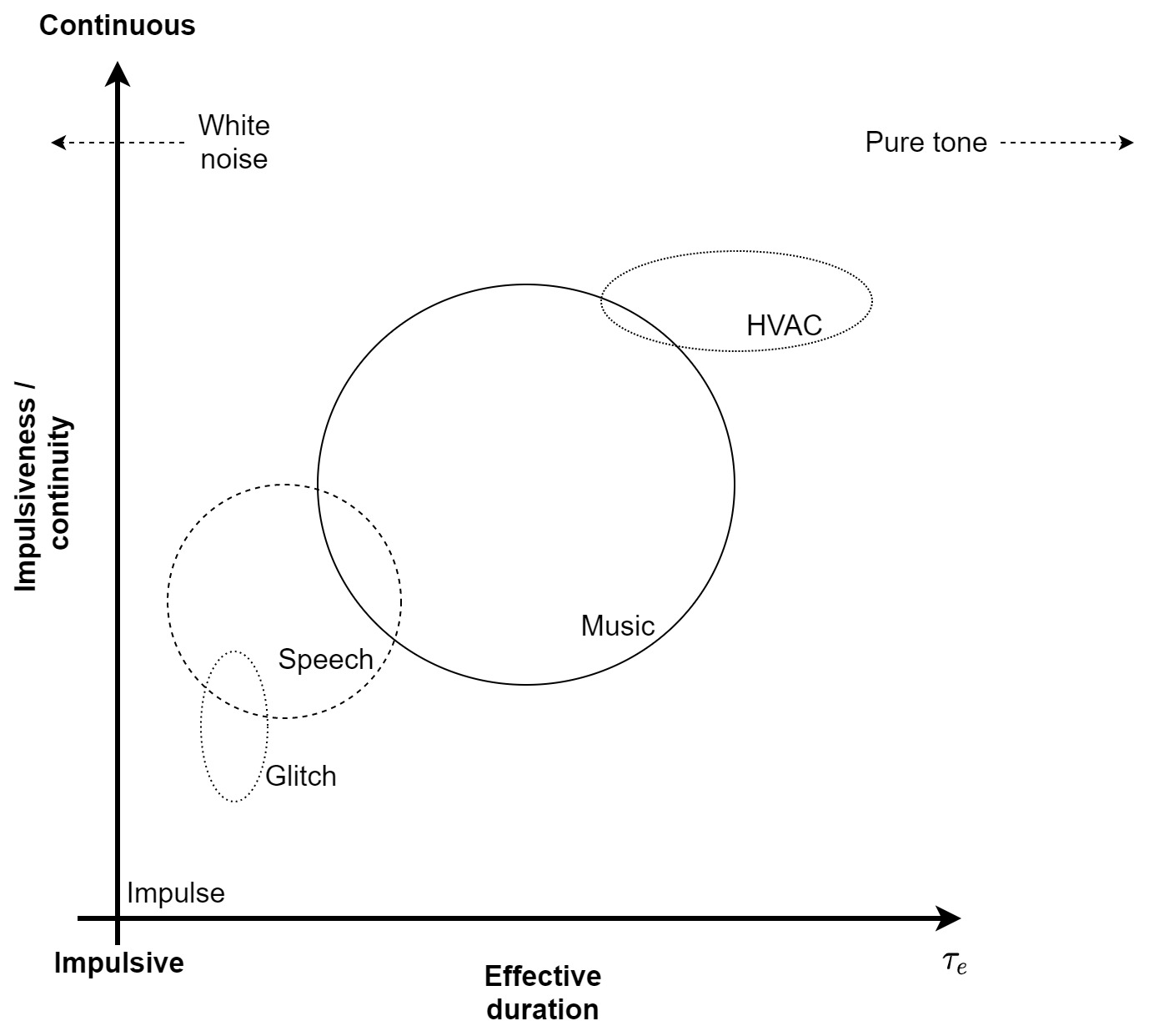
Figure 8.4: The rough relative range of the effective duration of different types of acoustic signals and their impulsiveness. This is drawn according to D'Orazio and Garai (2017, Figures 4), with slight modifications.

8.3.3 Coherence time of realistic sources

Given the relative lack of narrowband coherence data in literature, several additional acoustic sources were analyzed in §A. The results show the interactions between coherence and the spectral features in the analyzed channel, the instantaneous tonality, and the type of source. Sources that have sustained and resonant normal modes are more coherent than transient sources, including speech. However, the variability is very large, and becomes even larger when it interacts with the room acoustics.

One immediate observation is that coherence time values are long at lower frequencies and are almost always very short at high frequencies (i.e., above 2000 Hz). This can be due to the narrowband filtering and the sources themselves. The analysis filters impose some coherence on the signals, which is proportional to the absolute bandwidth of the filter, rather to its relative bandwidth (Eqs. 8.31 and 8.71). Since filter banks (including the cochlear one) tend to have a relatively small variation in the relative bandwidth as a function of frequency, then high frequencies that are analyzed by them will always be less coherent, by the definition of coherence time. Therefore, inasmuch as the filters themselves have a cohering effect on the signals, it decreases with frequency. Perhaps more importantly, the acoustic sources surveyed were musical and human sounds, which tend to be well-tuned only at low frequencies. At high frequencies, their high modal density may preclude stable narrowband sounds with the filters used. As the survey of sources was anything but exhaustive, more data will have to be analyzed in the future to enable a better grasp of these issues.

Audio demos are available for some of the samples used in the experiment, which may be informative for the reader to get a handle of the different coherence regimes—especially when heard along with the various plots in §A.

8.3.4 Discussion

The combined data from literature and from §A are sufficient to give an idea about the ranges of coherence times associated with different sources. Importantly, they enable us to relate to a continuum of coherence times, which may be indicative of the subjective perception of coherent, partially coherent, and incoherent sources. As a rule, natural sources are rarely completely coherent or completely incoherent, but sources with coherence time on the order of a couple of milliseconds or less will be assumed incoherent, whereas those in the hundreds of milliseconds will be assumed coherent. These bounds will demarcate the relevance of acoustic and auditory phenomena that can be explained by interference.

A common theme in this chapter and the rest of this work is that realistic acoustic sources and fields are partially coherent. Now that we have the extreme bounds of coherent and incoherent sources—what sounds could count as partially coherent? As was shown earlier (Eq. 8.21), partial coherence can be expressed as a sum of completely coherent and completely incoherent contributions that are weighted by \(|\gamma|\) and \(1-|\gamma|\), respectively. Furthermore, according to Eq. 8.22, \(|\gamma|=0.5\) when the coherent and incoherent contributions are equal. For a purely temporal coherence measurement, this equality is satisfied exactly at the coherence time \(\tau = \Delta \tau\), namely, at the full-width half-maximum of the coherence distribution.

As a rule of thumb we shall consider the completely coherent regime of a coherence function to be contained within the coherence time interval \(|\tau| \geq \Delta\tau\). Similarly, the completely incoherent regime will be outside of the effective duration \(|\tau| \leq \tau_e\). The partially coherent regime is going to be everything in the middle \(\Delta\tau \leq |\tau| \leq \tau_e\), which leaves some room for ambiguity that may depend on the individual responses and their interaction with the particular source.

Note that even though we have discussed the results based on autocorrelation (self-coherence), it does not imply that such an operation is necessarily being performed within the auditory system—something that has been questioned in literature (Loeb et al., 1983; Kaernbach and Demany, 1998). Rather, autocorrelation here is the mathematical tool that reveals what kind of acoustic source is being radiated. This information affects the receiver whether or not it has a physiological autocorrelator. See §8.6 for further discussion about autocorrelation in the auditory system.

8.4 Decoherence through reflections and reverberation

Out of all the branches of acoustics, room acoustics may have made the most extensive use of stochastic tools that have parallels in scalar electromagnetic coherence theory (§7.2.3). This is because reverberation is most effectively described as an ensemble of reflections with random phase, whereas a complete solution of the wave equation for all room modes becomes untenable at high frequencies, where the modal density of the room is prohibitively high. The fundamental effect of reverberation on coherence is to gradually decohere the sounds through reflections, spectral broadening, and mixing with numerous other reflections in the field. Therefore, the reverberant sound field is usually divided into two limiting cases—the coherent/direct sound and the incoherent/reflected sound (Morse and Bolt, 1944). The details matter, though, as the source type, boundary (room) structure, and construction materials determine the extent of decoherence that is ultimately detected by the ears. While the topic of room acoustics is too large to fully reframe in light of coherence theory, several basic results will be reviewed below that will provide the foundation for later analysis of the auditory system response to signals in their everyday environments.

8.4.1 Coherence and reflections

A complete description of the pressure waves reflected from a surface can be prohibitively complex and only relatively simple cases can be solved analytically (see §3.4.3). The coherence approach avoids this difficulty by looking only at the relative point-to-point transformation of the wave function and at its potential to cause interference, rather than at a complete description of the entire field. This is particularly useful because any one-dimensional field function—fully describable as point source and point receiver (as is the effective pressure field arriving in each ear)—may be fully characterized by its instantaneous amplitude and phase (see §3.5).

Following the propagated field from a source with a known degree of coherence, we would like to know how its radiated pressure changes as a result of reflections. We can make a few inferences based on §3.4.3. In the simplest case, a hard wall of very large dimensions (with respect to the longest wavelength of the sound field) acts as a perfect mirror. The pressure at any point in front of the wall is a superposition of the direct sound and its reflection from the wall. The time delay of the reflection that corresponds to \(\tau\) in the coherence function \(\gamma(\tau)\) is determined by the distance from the wall, the angle of incidence, and the wall impedance. If \(\tau\) is smaller than the coherence time of the source, then the direct and reflected sounds interfere and level variations will be measurable around the point, embodying the interference fringes in the acoustic field. When the time delay is not much larger than the coherence time, partial coherence leads to partial interference that exhibits poor fringe visibility (measured in space). Finally, when the wall is not hard, then the reflected wave is generally attenuated and exhibits a frequency-dependent phase response, which can also lead to a loss of coherence (if the source is not monochromatic), even when the associated time delay is well below the coherence time. Partially coherent broadband sound that is mixed with its reflection will exhibit spectral ripples, or spectral modulation. Such ripples were observed in various geometrical configurations, where the source was placed between two, three, or four reflecting walls in Berman (1975). Even though the source was coherent (pure tones), the spectrum was affected by the modes that existed between the walls, which gave rise to a complex interference pattern that is seen in the spectrum.

8.4.2 Coherence and reverberation

Reverberation is caused by the ensemble of reflections between an acoustic source and its environment, which arrive to a receiver asynchronously. The reflected waves are further reflected between surfaces until the reflected energy eventually becomes fully dissipated and the sound dies out. The delay associated with each discrete reflection is determined by the distance from the source, angle of incidence, and the surface impedance—summed over multiple reflections. Reverberation can be statistically characterized using its reverberation time, which is proportional to the duration of the sound decay in the reverberant space. In its simplest formulation⁸⁰, the reverberation time is a function of the total surface area \(\mathit{S}\), its relative absorption \(0 \leq \mathit{\alpha} \leq 1\) (0 is completely absorbent, 1 completely reflective), and the volume \(V\) of the space—through Sabine's formula (Sabine, 1923):

\[ T_{60} = 6\ln 10 \cdot \frac{4V}{c\mathit{S \alpha}} \]

(8.85)

Technically, it is defined as the time it takes for stationary sound to drop by 60 dB (to one millionth of its original level) from when it is switched off. Nowadays, it is usually evaluated directly from the impulse response function of the space. Although reverberation has been explored mainly inside built rooms, its applicability is completely general to other spaces with enough reflective surfaces to elicit statistical behavior (see §3.4.4). Therefore, the reference to rooms provides a convenient system that is also relevant to much of humanity, but many of the conclusions most certainly go beyond built enclosures.

The validity of the statistical approach to reverberation largely depends on how random the sound field is—a property which is captured by the diffuse field model. The diffuse field has been a highly useful theoretical model for investigating the effects of reverberation. In a perfectly diffuse field, the number of reflections, their phase, and their direction are completely random (the quantities are average, so the randomness is evaluated over time) and behave ergodically (Morse and Bolt, 1944). Jacobsen (1979, p. 12, definition II with interpretation B) explored several related definitions for a diffuse field in a reverberation chamber and zeroed in on: “A diffuse sound field comprises an infinite number of plane propagating waves with random phase relations, arriving from uniformly distributed directions.” And additionally, “At an arbitrary position in a pure-tone field the phase relations of the waves constitute a fixed set of random variables.” These somewhat technical definitions have been mainly used with spectral coherence, although it was developed independently from that reviewed in §8.2.7.

A room that approximates a diffuse field is called a reverberation chamber. It is notionally antonymous to the anechoic chamber, whose design goal is to approximate free-field behavior that renders exclusive the direct sound from the acoustical source by minimizing reflections through heavy absorption (Kuttruff, 2017; pp. 151–154 and 221–225). In interpreting experimental acoustic data, it is perhaps handy to consider the following analogies. The diffuse field is to spatial coherence what white noise is to temporal coherence—both approach the limit of complete incoherence with infinitesimally small spatial or temporal shifts in their respective self-coherence functions. Similarly, the free field is to spatial coherence what the pure tone is to temporal coherence—both approach the limit of complete coherence with infinitesimally large spatial and temporal shifts in their respective self-coherence functions. As always, reality lies somewhere in between these idealized model fields, as Morse and Bolt (1944) admitted that “...room acoustics finds itself in the difficult intermediate region,” referring to the gulf between statistical modeling of rooms using geometrical acoustics and accurate modeling with wave acoustics that is often impractical. In a similar vein, Kinsler et al. (1999, p. 140) commented on the difference between coherent and incoherent summation of a monochromatic source: “A typical case of continuous wave propagation may lie somewhere between these two idealizations. Coherence is favored by short-range, low-frequency, smooth boundaries, few boundary reflections, and a stable and smooth speed of sound profile. Random phasing is favored by the converse conditions.”

It becomes valid to model an acoustic field as diffuse where the enclosure supports a high modal density with respect to frequency. This is the case for large rooms, as is expressed by the Schroeder cross-over frequency (Schroeder, 1996)

\[ f \approx 2000 \sqrt{\frac{T_{60}}{V}} \,\,\, \mathop{\mathrm{Hz}} \]

(8.86)

for \(T_{60}\) measured in s and \(V\) in \(\mathop{\mathrm{m}}^3\). This formula guarantees that frequencies above \(f\) resonate due to at least three normal room modes, on average—so no normal mode “isolates” are allowed. Below the cross-over frequency, single modes may dominate the response, which is no longer well-described by statistical considerations. By inverting Eq. 8.86 and turning it into an inequality, we can relate to “large rooms” with an approximate diffuse field if they have a volume \(V > T_{60}(2000/f)^2\) (Kuttruff, 2017; p. 68). In contrast, “small rooms” may not have a meaningful \(T_{60}\) associated with them, because individual normal modes occupy significant bandwidths. However, \(T_{60}\) is generally dependent on frequency, so its blanket application in all these formulas requires caution.

Despite its power as a theoretical tool, the diffuse field approximation is often violated in real rooms and should only serve as a limiting case (Morse and Bolt, 1944; Waterhouse, 1968). There are correlations in the diffuse sound field that demonstrate the limits of its randomness, which therefore induce extended coherence volumes than theory predicts⁸¹. For example, Waterhouse (1955) showed both theoretically and empirically that interference is observable along the room boundaries even in a highly reverberant chamber. The interference is constructive close to the boundary with the strongest effect for a corner, followed by an edge, and finally a wall that has the weakest effect. Naturally, the interference is most pronounced for coherent sources, as pure tone fringes are measurable up to a distance of a couple of wavelengths from the walls. With broadband noise, the effect decreases with increasing bandwidth, as its coherence length drops (see Eq. 8.37; Waterhouse, 1955; Figure 7). Even far away from the room boundaries, the spatial coherence of the diffuse broadband pressure field at two points is finite. Thus, an interference pattern can be observed, especially at low frequencies, given by the spatial coherence

\[ \mu(\boldsymbol{\mathbf{r_1}},\boldsymbol{\mathbf{r_2}},\omega) = \mathop{\mathrm{sinc}} \left( \frac{\omega |\boldsymbol{\mathbf{r_1}}-\boldsymbol{\mathbf{r_2}}|}{c} \right) \]

(8.87)

where \(\boldsymbol{\mathbf{r_1}}\) and \(\boldsymbol{\mathbf{r_2}}\) are the two measurement points (Cook et al., 1955). This formula was found to be correct also in rectangular rooms as long as the reverberant field is undamped, modal eigenfrequencies are unique, and the modal density is high enough to be approximated as continuous (Morrow, 1971).

Just as correlations exist in the temporal and spatial domains, they also characterize the spectral domain in the diffuse field. Sound components in the spectral domain are not entirely incoherent in large reverberant rooms. Schroeder (1962) showed that if the frequency response between two points is modeled as a random process, then the autocorrelation of the power spectrum (defined as a function of spectral distance \(|\omega_1-\omega_2|\)), goes as

\[ \mu(\boldsymbol{\mathbf{r}},\omega_1,\omega_2) = \frac{1}{1 + \left(\frac{|\omega_1-\omega_2| T_{60}}{13.8}\right)^2} \]

(8.88)

which we associated with the spectral nonstationary self-coherence function \(\mu\). The factor \(T_{60}/13.8\) represents the time it takes for an impulse to decay to a value of \(1/e\) from its initial value. The autocorrelation drops by about 10 dB for \(|f_1-f_2| = 6.6/T_{60}\), so that it takes the frequency spacing of a few Hertz for two components to become completely incoherent. A very similar result was obtained for the pressure amplitude autocorrelation function. Eq. 8.88 is a neat illustration of the decohering effect of reverberation—the longer the reverberation time is, the more decorrelated adjacent spectral components become, as the field becomes closer to a theoretically stationary field in which frequencies are incoherent (Eq. 8.29). However, caution must be taken when the spectral resolution of the measurement is higher than the spacing condition for incoherence, because the measurement filter can make the coherence appear higher than it is in reality (Jacobsen and Nielsen, 1987; Jacobsen and Roisin, 2000). Some examples of spectral coherence at different measurement points in a room are given in §A.6.3, where it is shown that realistic sources can be much more spectrally correlated in standard (non-diffuse) rooms than is predicted by Eq. 8.88.

At the sound receiver in the reverberant space, three coherence regimes may be noticeable—two distinct and one that is more elusive. First, the direct sound from the source arrives uninterrupted to the receiver before the first reflection does. When the source is coherent, then its mutual coherence function is largely retained in this duration, as it propagates according to the wave equation (Eqs. 8.41 and 8.42) and does not suffer from the decohering effects of reflection (8.4.1). Second, if a certain surface is much closer to the receiver than other surfaces, then a single reflection may interfere with the direct sound, if the direct sound and reflection are both coherent. Additional “early reflections” are possible over a short time window that produce some interference, depending on the surrounding geometry⁸². Third, late reflections are no longer distinct and they arrive with random phases, which add incoherently in intensity without interfering. The first and third regimes can be distinguished by noting that the power of the reverberant field is independent of position and constitutes a constant fraction of the source power. Thus, a room may be characterized by the distance in which the direct and reverberant powers are equal—the critical distance or the diffuse-field distance (Kuttruff, 2017; p. 118)

\[ r_c \approx 0.1 \sqrt{\frac{V}{\pi T_{60}}} \]

(8.89)

The separation between the early and late reflection regimes may not be clear-cut. Rarely, a distant and high-level reflection can stick out as an echo that is a distinct coherent reflection within the incoherent reverberant tail. A more common coherent effect may be a series of regular reflections that are caused by structural geometrical regularities such as parallel walls or spherical domes, which can give rise to flutter echo and/or coloration. These are modulation effects, which are imposed as peaks in the coherence function (either spectral or temporal) of the sound pressure in the room (see §3.4.4).

The various effects of reverberation on radiated sound are of major importance in hearing, as they represent every possible degree of coherence that has to be dealt with by the hearing system. Stationary signals are of rather limited usefulness in everyday listening, especially when information transfer is considered, which contains modulations that can be on the temporal scale of the temporal fluctuations of the field itself. When the sound source is continuous but nonstationary, “fresh” direct sound is continuously mixed with the early and late reflections of previously emitted sound. In this case, if the source is highly coherent, the early reflections are dominant, and the source variation is rapid, then new and old information from the source can interfere and make any message communication difficult. Also, when the reverberation time is long—its energy decays slowly—it produces an approximately constant intensity level that “washes out” or reduces the contrast of fresh acoustic information (or the modulation depth in amplitude modulation; Houtgast and Steeneken, 1973).

A few examples for some of the above effects are provided in §A. In brief, they illustrate how realistic room acoustics produces a partially coherent field that varies in time, space, and frequency, and depends on the acoustic content of the source and on the reverberant space. The analysis also demonstrates how typical signals are generally nonstationary and it is often not straightforward to predict how a signal is affected by reverberation in a field that is not ideally diffuse. Nevertheless, statistical effects that are predicted for stationary sounds in diffuse fields are occasionally observed, locally.

8.5 Interaural coherence

We will be remiss without mentioning the binaural function, which can be readily included in the general framework of coherence theory. Interaural cross-correlation between the two ear signals has been originally proposed by Licklider (1948) as a means to separate speech from broadband noise that the hearing system employs. Diotic speech intelligibility significantly improved when either the noise or the speech was out of phase between the two ears, while the other was in phase. The advantage was retained for partial coherence of the noise \(\gamma(R, 0) \leq -0.75\) for in-phase speech or \(\gamma(R, 0) \geq 0.75\) when it was out of phase, where we set \(R = |\boldsymbol{\mathbf{r_1}} - \boldsymbol{\mathbf{r_2}}|\) to be the fixed distance between the two ears of the listener. Another effect is of the perceived size of the acoustic source—its apparent source width in the listener's “phenomenal space”—turns out to also be a function of the interaural coherence (Licklider, 1948). It was shown to be a quantity that listeners are very sensitive to (down to the \(|\gamma| = 0.1\) level; Jeffress et al., 1962). Other effects can be at least partially explained by interaural correlation, such as perceived binaural loudness, binaural beats, and the binaural “Huggins” pitch.

The spatial coherence function of the head interacts with the room acoustics. Lindevald and Benade (1986) presented coherence data of a person walking in a reverberant field (\(T_{60} \approx 1\) s) of a large lecture hall (\(V=1000\) \(\mathop{\mathrm{m}}^3\)) that had a loudspeaker playing sinusoidal tones. The interaural coherence was clearly affected by the head shadow and the two ear signals became incoherent at a frequency as low as 500 Hz (the first zero of a sinc function). When the measurement was repeated for two microphones spaced as the two ears (\(R = 15\) cm), the first zero was reached at 1100 Hz, so the response was more coherent. Thus, the head has a measurable spatially decohering effect on the sound field.

Binaural research has not formally engaged with coherence theory beyond the interaural-correlation. The one (informal) exception to this is Cohen (1988), who proposed that the interaural function is, in fact, an interferometer (see also Dietz and Ashida, 2021). This idea can be readily developed using the theory we presented earlier in the chapter. In principle, the classical duplex cues for binaural localization—interaural time difference (ITD) and interaural level difference (ILD) (Rayleigh, 1907b)—may be recast as elements within the interaural coherence function. The ILD relates to the level difference, which leads to partial incoherence and audibility of less than unity (Eq. 8.19).

The ITD relates to delay—a constant phase term in the cross-term of the coherence function (i.e., \(\delta\) in Eqs. 8.13 and 8.14). Substantial efforts have been dedicated to modeling physiological mechanisms that fulfill the role of coincidence detectors—neurons with two excitatory inputs that fire only when the binaural inputs are synchronized and perform an instantaneous cross-correlation operation. It has been proposed that coincidence detectors are accompanied by matching signal processing that can extract the necessary information (Jeffress, 1948; Licklider, 1951b; Colburn, 1973; Colburn, 1977; Loeb et al., 1983; Shamma et al., 1989). While in reality the interactions and deviations from such a clean interpretation of the binaural operation are messy (e.g., Buchholz et al., 2018), there is recent physiological evidence from simultaneous juxtacellular recordings that the simple coincidence model may be sufficient to explain ITDs (Plauška et al., 2016). Regardless of the precise mechanism for computing the correlation, the effectiveness of using it to predict binaural unmasking has been found to be very high, for a host of listening stimuli and conditions (Encke and Dietz, 2022).

8.6 Coherence processing in the brain

Several models of pitch and harmonicity perception hypothesized brainstem circuitry that contains coincidence detectors that are not necessarily used in binaural processing. The important aspect about their operation is that they more-or-less instantaneously respond to input coherence, which means that their operation is adapted to nonstationary coherence by definition.

For example, Loeb et al. (1983) posited a cross-correlation function, explicitly within the brainstem—in particular in the medial superior olive (MSO)—that can work either monaurally or binaurally. According to this model, the spectral resolution of the ear can be explained using coincidence detectors that receive inputs from channels whose spectral distance corresponds to 0.3–0.4 of the respective wavelength on the basilar membrane. This model does not resort to delay lines—a signal processing component that was hypothesized by Jeffress (1948) that may be valid in birds, but probably not in mammals (Grothe et al., 2010). Shamma and Klein (2000) hypothesized that a matrix of coincidence detectors may be responsible for harmonicity perception and various types of pitch (periodicity and residue), which are not easily explained without a cross-correlation setup that includes delay lines (for which there is no clear evidence). The model requires phase locking (see §9.7.2) and distortion products (obtained through squaring) to have the information necessary for synchronization within the channel. It also hypothesizes spectral and temporal sharpening and that the inherent dispersion between the channels is necessary for eliciting their synchronization later in processing, regardless of the signal type. A related model by Carney et al. (2002) proposed a coincidence detector network that can detect pitch in noise. The network comprises all the adjacent channels that are affected by the stimulus and individually phase lock. Roughly, the idea here is that when sound elements coincide, they add up coherently and produce a sharp frequency response, whereas the noise is broad and does not add cumulatively to the sharpness of its spectrum. The model requires for specific phase relations to exist between adjacent channels. As a final example, the model by Langner (2015) identified periodicity mapping (periodopy) at the central nucleus of inferior colliculus (ICC), which is orthogonal to its tonotopy. In this model, the unique mesh-like topology of ICC neurons enables them to work as coincidence detectors for spikes that arrive from the dorsal and ventral cochlear nuclei (delayed), and the ventral nucleus of the lateral lemniscus (inhibition) (see Figures in Langner, 2015, pp. 129 and 168).

8.7 Discussion

Basic principles of coherence theory that are germane to acoustics and hearing science were reviewed above. While perhaps none of the ideas presented in this chapter are new to the field, they have never been presented en masse in this context in a comprehensive and rigorous manner. Nevertheless, acoustic coherence is intimately related to the identity of sound sources, which the auditory system can detect and react to. Later in this work, it will become apparent that the auditory system is inherently set up to differentially process coherent and incoherent stimuli, so the basic distinction between them is critical. Because every partially-coherent stimulus can be expressed as a sum of coherent and incoherent components, such a decomposition potentially endows the system with a unique handle to identify and process different sound sources.

The review dwelt on room acoustic effects, which were originally described using stationary signals in diffuse sound fields. These are generally not representative of most common acoustic stimuli, as was demonstrated in §8.3.2 and §A for a handful of human and musical sources. As these signals arrive to the outer ear and propagate to the cochlea via the middle ear, it can be expected that their coherence function will vary within the ear as well, albeit only slightly due to the very small distances involved. Things are more complex inside the cochlea because of dispersion, phase locking, and discretization, as will be discussed in subsequent chapters.

It is important to make a distinction between signal processing that requires coherence detection as part of the computation and coherence that is propagated within the system, which represents an inherent property of the signal. Coincidence detectors are of the first kind, whereas other references to coherence in the brain (e.g., temporal self-coherence or autocorrelation) may be a propagated property of the second kind. The latter is the most important type of coherence in the present context, because it is an inherent feature of the signal that directly corresponds to its wave nature. Removing coherence from the signal is tantamount to removing some information that it carries about its source. Therefore, for coherence to not propagate into the auditory brain may be just as nontrivial a processing step as the opposite case. In the next chapter we will focus mainly on phase locking as a feature that facilitates coherence propagation.

Footnotes

71. More advanced theory deals with polarization effects as well, which are of no relevance in acoustics. The classical domain is sufficient to explain most imaging effects, but an extensive quantum coherence theory has also been developed. See Mandel and Wolf (1995).

72. A random or stochastic process relates to a variable or variables that are drawn from a certain probability distribution. Without getting into any mathematical formalities, whenever we discuss arbitrary signals or waves, they can be modeled as a random process, which facilitates certain types of analyses. Stochastic processes are distinguished from deterministic processes. See the cited literature in §8.1 for more formal short introductions. For an extensive introduction, see, for example, Bendat and Piersol (2011). For a shorter introduction, see Middleton (1996).

73. Two general types of stationary processes are distinguished. A strict-sense stationary process is defined to be independent of time. Thus, such a process can be sampled at any time point without affecting the average. White noise is the simplest such process. A wide- or weak-sense stationary process has a constant average, and a time-invariant cross-correlation function, which depends only on the time difference and not on the absolute time points of the process. Wide-sense stationarity requires that the second moments of the process exist. In the text, whenever stationarity is invoked, it is meant in the wide sense.

74. When applied to pressure waves, the term audibility will be more appropriate than visibility, or the more neutral term contrast, as audibility is often used in hearing to designate that a stimulus or a manipulation thereof is above the individual's threshold. However, visibility is the more standard term in optics and we will used it below.

75. Jacobsen and Nielsen (1987) made the distinction that the acoustic correlation function is bandlimited, whereas the coherence is defined in the frequency domain.

76. We have dispensed with the formal discussion of harmonizable random processes due to Loève that is usually invoked here and may be relevant to the discussion of the analytic signal (§6). In general, it deals with nonstationary random processes with infinite energy that may also be discontinuous, for which the standard Fourier transform does not exist—only the power spectrum via the autocorrelation function (see §8.2.3). Instead, it then applies the Riemann-Stieltjes integral for the spectral density, \(x'(t) = \frac{1}{2\pi}\int dX(\omega) e^{i\omega t}\). For further details, see Clark (2012, pp. 173–178) for a friendly and brief introduction, or for a more complete treatment Napolitano (2012).

77. The conditions are that the cross-spectral matrix \(W(\boldsymbol{\mathbf{r_1}},\boldsymbol{\mathbf{r_2}},\omega)\) is non-negative, definite, and Hermitian. These conditions make it suitable for expansion into eigenfunctions (Eq. 8.47) according to Mercer's theorem. In this case, the modes satisfy the Fredholm equation (8.46) for which \(W\) is the kernel.

78. Before the advent of laser technology, the alternative in optics has been to use a monochromator, which produces a narrowband spectrum from a broadband light source. This is usually achieved by spatially selecting the diffracted or dispersed product of the broadband light. This technology is still widely used in applied optics.

79. In the paper the coherence time is referred to simply as the width of the autocorrelation peak and is notated with \(W_{\phi(0)}\).

80. For a brief review of alternatives and limitations see Xiang (2020).

81. The coherence volume is defined as an extension to coherence length in three dimensions, as the volume around a point in which interference may be observed (Wolf, 2007; pp. 8–10). The concept is not used in acoustics, but seems appropriate in the context of three-dimensional fields.

82. It is common to distinguish between specular and diffuse reflectors in this context. Specular reflections tend to be coherent, as they may give rise to interference between the incident and reflected sounds. The reflectors are usually hard and flat surfaces with no discontinuities. In contrast, a diffuse reflector (a diffuser) is designed to emulate a more randomized phase response as much as possible and thereby decohere the reflected sound and minimize interference effects. It therefore attempts to maximize the surface geometrical randomness and discontinuities in order to decohere the impinging field. Cox and D'Antonio (2005, p. 30–31) noted that strictly speaking all passive reflectors are coherent, because they are time invariant and deterministic. They additionally noted that the effect of diffusers is then better thought of as temporal and spatial dispersion of the field and not of decoherence.

References

Aertsen, AMHJ, Olders, JHJ, and Johannesma, PIM. Spectro-temporal receptive fields of auditory neurons in the grassfrog. I. Characterization of tonal and natural stimuli. Biological Cybernetics, 38 (3): 223–234, 1980b.

Aertsen, AMHJ, Johannesma, Peter IM, and Hermes, DJ. Spectro-temporal receptive fields of auditory neurons in the grassfrog. II. Analysis of the stimulus-event relation for tonal stimuli. Biological Cybernetics, 38 (4): 235–248, 1980a.

Aertsen, AMHJ and Johannesma, PIM. The spectro-temporal receptive field: A functional characteristic of auditory neurons. Biological Cybernetics, 42 (2): 133–143, 1981.

Ando, Yoichi and Alrutz, Herbert. Perception of coloration in sound fields in relation to the autocorrelation function. The Journal of the Acoustical Society of America, 71 (3): 616–618, 1982.

Ando, Yoichi. Concert Hall Acoustics. Springer-Verlag, Berlin, Germany, 1st edition, 1985.

Ando, Yoichi. Architectural Acoustics: Blending Sound Sources, Sound Fields, and Listeners. Springer-Verlag, NY, New York, 1998.

Ando, Yoichi and Cariani, Peter. Auditory and Visual Sensations. Springer Science+Business Media, LLC, New York, NY, 2009.

Antoni, Jérôme. Cyclostationarity by examples. Mechanical Systems and Signal Processing, 23 (4): 987–1036, 2009.

Bastiaans, Martin J. A frequency-domain treatment of partial coherence. Optica Acta: International Journal of Optics, 24 (3): 261–274, 1977.

Bendat, Julius S and Piersol, Allan G. Random Data: Analysis and Measurement Procedures. John Wiley & Sons, Hoboken, NJ, 4th ed. edition, 2011.

Berman, JM. Behavior of sound in a bounded space. The Journal of the Acoustical Society of America, 57 (6): 1275–1291, 1975.

Berman, David H and McCoy, John J. Coherence propagation and geometric acoustics. The Journal of the Acoustical Society of America, 79 (3): 635–643, 1986.

Bertolotti, Mario, Ferrari, Aldo, and Sereda, Leonid. Coherence properties of nonstationary polychromatic light sources. Journal of the Optical Society of America B, 12 (2): 341–347, 1995.

Born, Max, Wolf, Emil, Bhatia, A. B., Clemmow, P. C., Gabor, D., Stokes, A. R., Taylor, A. M., Wayman, P. A., and Wilcock, W. L. Principles of Optics. Cambridge University Press, 7th (expanded) edition, 2003.

Buchholz, Jörg M, Le Goff, Nicolas, and Dau, Torsten. Localization of broadband sounds carrying interaural time differences: Effects of frequency, reference location, and interaural coherence. The Journal of the Acoustical Society of America, 144 (4): 2225–2237, 2018.

Carney, Laurel H, Heinzy, Michael G, Evilsizer, Mary E, Gilkeyz, Robert H, and Colburn, H Steven. Auditory phase opponency: A temporal model for masked detection at low frequencies. Acta Acustica united with Acustica, 88 (3): 334–347, 2002.

De Cheveigné, Alain and Kawahara, Hideki. Yin, a fundamental frequency estimator for speech and music. The Journal of the Acoustical Society of America, 111 (4): 1917–1930, 2002.

Clark, Charles Pascal. Coherent demodulation of nonstationary random processes. PhD thesis, University of Washington, 2012.

Cohen, N. The interferometer paradigm for mammalian binaural hearing. In Bioastronomy – The Next Steps. Proceedings of the 99th colloquium of the international astronomical union, Balaton, Hungary, 1987, pages 235–235. Springer, 1988.

Colburn, H Steven. Theory of binaural interaction based on auditory-nerve data. I. General strategy and preliminary results on interaural discrimination. The Journal of the Acoustical Society of America, 54 (6): 1458–1470, 1973.

Colburn, H Steven. Theory of binaural interaction based on auditory-nerve data. II. Detection of tones in noise. The Journal of the Acoustical Society of America, 61 (2): 525–533, 1977.

Cook, Richard K, Waterhouse, RV, Berendt, RD, Edelman, Seymour, and Thompson Jr, MC. Measurement of correlation coefficients in reverberant sound fields. The Journal of the Acoustical Society of America, 27 (6): 1072–1077, 1955.

Cox, Trevor J. and D'Antonio, Peter. Acoustic Absorbers and Diffusers: Theory, Design and Application. Spon Press, Taylor & Francis Group, 2005.

D'Orazio, Dario and Garai, Massimo. The autocorrelation-based analysis as a tool of sound perception in a reverberant field. Rivista di Estetica, 66: 133–147, 2017.

Derode, Arnaud and Fink, Mathias. The notion of coherence in optics and its application to acoustics. European journal of physics, 15 (2): 81, 1994.

Dietz, Mathias and Ashida, Go. Computational models of binaural processing. In Litovsky, Ruth Y., Goupell, Matthew J., Fay, Richard R., and Popper, Arthur N., editors, Binaural Hearing, volume 73, pages 281–315. Springer Nature Switzerland AG, Cham, Switzerland, 2021.

D'Orazio, Dario, De Cesaris, Simona, and Garai, Massimo. A comparison of methods to compute the "effective duration"� of the autocorrelation function and an alternative proposal. The Journal of the Acoustical Society of America, 130 (4): 1954–1961, 2011.

Encke, Jörg and Dietz, Mathias. A hemispheric two-channel code accounts for binaural unmasking in humans. Communications Biology, 5 (1): 1122, 2022.

Fourdouiev, V. Évaluation objective de l'acoustique des salles. In Proceedings of 5th International Congress on Acoustics, Liege, Belgium, pages 41–54, 1965.

Fujii, Kenji, Soeta, Yoshiharu, and Ando, Yochi. Acoustical properties of aircraft noise measured by temporal and spatial factors. Journal of Sound and Vibration, 241 (1): 69–78, 2001.

Gabor, Dennis. Theory of communication. Part 1: The analysis of information. Journal of the Institution of Electrical Engineers-Part III: Radio and Communication Engineering, 93 (26): 429–457, 1946.

Goodman, Joseph W. Statistical optics. John Wiley & Sons, Inc., Hoboken, NJ, 2nd edition, 2015.

Grothe, Benedikt, Pecka, Michael, and McAlpine, David. Mechanisms of sound localization in mammals. Physiological Reviews, 90 (3): 983–1012, 2010.

Havelock, David I, Stinson, Michael R, and Daigle, Gilles A. Measurements of the two-frequency mutual coherence function for sound propagation through a turbulent atmosphere. The Journal of the Acoustical Society of America, 104 (1): 91–99, 1998.

Hillenbrand, James. Perception of aperiodicities in synthetically generated voices. The Journal of the Acoustical Society of America, 83 (6): 2361–2371, 1988.

Houtgast, T and Steeneken, H JM. The modulation transfer function in room acoustics as a predictor of speech intelligibility. Acta Acustica united with Acustica, 28 (1): 66–73, 1973.

Jacobsen, Finn. The diffuse sound field: Statistical considerations concerning the reverberant field in the steady state. PhD thesis, Acoustics Laboratory, Technical University of Denmark, 1979.

Jacobsen, Finn and Nielsen, TG. Spatial correlation and coherence in a reverberant sound field. Journal of Sound and Vibration, 118 (1): 175–180, 1987.

Jacobsen, Finn. Active and reactive, coherent and incoherent sound fields. Journal of Sound and Vibration, 130 (3): 493–507, 1989.

Jacobsen, Finn and Roisin, Thibaut. The coherence of reverberant sound fields. The Journal of the Acoustical Society of America, 108 (1): 204–210, 2000.

Jeffress, Lloyd A. A place theory of sound localization. Journal of Comparative and Physiological Psychology, 41 (1): 35, 1948.

Jeffress, Lloyd A, Blodgett, Hugh C, and Deatherage, Bruce H. Effect of interaural correlation on the precision of centering a noise. The Journal of the Acoustical Society of America, 34 (8): 1122–1123, 1962.

Kaernbach, Christian and Demany, Laurent. Psychophysical evidence against the autocorrelation theory of auditory temporal processing. The Journal of the Acoustical Society of America, 104 (4): 2298–2306, 1998.

Kawahara, Hideki, Masuda-Katsuse, Ikuyo, and De Cheveigné, Alain. Restructuring speech representations using a pitch-adaptive time–frequency smoothing and an instantaneous-frequency-based f0 extraction: Possible role of a repetitive structure in sounds. Speech Communication, 27 (3-4): 187–207, 1999.

Kinsler, Lawrence E, Frey, Austin R, Coppens, Alan B, and Sanders, James V. Fundamentals of Acoustics. John Wiley & Sons, Inc., New York, NY, 4th edition, 1999.

Kuster, Martin. Spatial correlation and coherence in reverberant acoustic fields: Extension to microphones with arbitrary first-order directivity. The Journal of the Acoustical Society of America, 123 (1): 154–162, 2008.

Kuttruff, Heinrich. Room acoustics. CRC Group, Taylor & Francis, Boca Raton, FL, 6th edition, 2017.

Lajunen, Hanna, Vahimaa, Pasi, and Tervo, Jani. Theory of spatially and spectrally partially coherent pulses. Journal of the Optical Society of America A, 22 (8): 1536–1545, 2005.

Lancis, Jesús, Torres-Company, Víctor, Silvestre, Enrique, and Andrés, Pedro. Space–time analogy for partially coherent plane-wave-type pulses. Optics Letters, 30 (22): 2973–2975, 2005.

Langner, Gerald D. The Neural Code of Pitch and Harmony. Cambridge University Press, Cambridge, United Kingdom, 2015.

Licklider, J. C. R. The influence of interaural phase relations upon the masking of speech by white noise. The Journal of the Acoustical Society of America, 20 (2): 150–159, 1948.

Licklider, Joseph Carl Robnett. A duplex theory of pitch perception. Experientia, 7 (4): 128–134, 1951b.

Lindevald, IM and Benade, AH. Two-ear correlation in the statistical sound fields of rooms. The Journal of the Acoustical Society of America, 80 (2): 661–664, 1986.

Loeb, Gerald E, White, Mark W, and Merzenich, Michael M. Spatial cross-correlation. Biological Cybernetics, 47 (3): 149–163, 1983.

Magyar, G and Mandel, L. Interference fringes produced by superposition of two independent maser light beams. Nature, 198 (4877): 255–256, 1963.

Mandel, Leonard and Wolf, Emil. Coherence properties of optical fields. Reviews of Modern Physics, 37 (2): 231, 1965.

Mandel, L and Wolf, E. Spectral coherence and the concept of cross-spectral purity. Journal of the Optical Society of America, 66 (6): 529–535, 1976.

Mandel, Leonard and Wolf, Emil. Optical Coherence and Quantum Optics. Cambridge University Press, Cambridge, United Kingdom, 1995.

Mark, William D. Spectral analysis of the convolution and filtering of non-stationary stochastic processes. Journal of Sound and Vibration, 11 (1): 19–63, 1970.

McCoy, JJ and Beran, MJ. Propagation of beamed signals through inhomogeneous media: A diffraction theory. The Journal of the Acoustical Society of America, 59 (5): 1142–1149, 1976.

Mehta, Dalip Singh, Saxena, Kanchan, Dubey, Satish Kumar, and Shakher, Chandra. Coherence characteristics of light-emitting diodes. Journal of Luminescence, 130 (1): 96–102, 2010.

Middleton, David. An Introduction to Statistical Communication Theory. IEEE Press, Piscataway, NJ, 1996. 2nd reprint edition; originally published in 1960.

Morrow, CT. Point-to-point correlation of sound pressures in reverberation chambers. Journal of Sound and Vibration, 16 (1): 29–42, 1971.

Morse, Philip M and Bolt, Richard H. Sound waves in rooms. Reviews of Modern Physics, 16 (2): 69, 1944.

Napolitano, Antonio. Generalizations of Cyclostationary Signal Processing: Spectral Analysis and Applications. John Wiley & Sons, Ltd., Chichester, United Kingdom, 2012.

Neeser, Fredy D and Massey, James L. Proper complex random processes with applications to information theory. IEEE Transactions on Information Theory, 39 (4): 1293–1302, 1993.

Picinbono, Bernard. On circularity. IEEE Transactions on Signal Processing, 42 (12): 3473–3482, 1994.

Picinbono, Bernard and Bondon, Pascal. Second-order statistics of complex signals. IEEE Transactions on Signal Processing, 45 (2): 411–420, 1997.

Plauška, Andrius, Borst, J Gerard, and van der Heijden, Marcel. Predicting binaural responses from monaural responses in the gerbil medial superior olive. Journal of Neurophysiology, 115 (6): 2950–2963, 2016.

Rayleigh, Lord. XII. On our perception of sound direction. The London, Edinburgh, and Dublin Philosophical Magazine and Journal of Science, 13 (74): 214–232, 1907b.

Sabine, Wallace Clement. Reverberation. In Collected Papers on Acoustics. Harvard University Press, Cambridge, MA, 2nd edition, 1923. “Reverberation” was published originally in “The American Architect”, 1900.

Schreier, Peter J and Scharf, Louis L. Stochastic time-frequency analysis using the analytic signal: Why the complementary distribution matters. IEEE Transactions on Signal Processing, 51 (12): 3071–3079, 2003.

Schroeder, Manfred Robert. Frequency-correlation functions of frequency responses in rooms. The Journal of the Acoustical Society of America, 34 (12): 1819–1823, 1962.

Schroeder, Manfred R. The ”schroeder frequency” revisited. The Journal of the Acoustical Society of America, 99 (5): 3240–3241, 1996.

Shamma, Shihab A, Shen, Naiming, and Gopalaswamy, Preetham. Stereausis: Binaural processing without neural delays. The Journal of the Acoustical Society of America, 86 (3): 989–1006, 1989.

Shamma, Shihab and Klein, David. The case of the missing pitch templates: How harmonic templates emerge in the early auditory system. The Journal of the Acoustical Society of America, 107 (5): 2631–2644, 2000.

Shimokura, Ryota, Akasaka, Sakie, Nishimura, Tadashi, Hosoi, Hiroshi, and Matsui, Toshie. Autocorrelation factors and intelligibility of japanese monosyllables in individuals with sensorineural hearing loss. The Journal of the Acoustical Society of America, 141 (2): 1065–1073, 2017.

Shin, Kihong and Hammond, Joseph. Fundamentals of Signal Processing for Sound and Vibration Engineers. John Wiley & Sons, West Sussex, England, 2008.

Verdet, Émile. Leçons d'optique physique, volume 1. Victor Masson et Fils, Paris, 1869.

Waterhouse, Richard V. Interference patterns in reverberant sound fields. The Journal of the Acoustical Society of America, 27 (2): 247–258, 1955.

Waterhouse, Richard V. Statistical properties of reverberant sound fields. The Journal of the Acoustical Society of America, 43 (6): 1436–1444, 1968.

Wiener, Norbert. Generalized harmonic analysis. Acta Mathematica, 55: 117–258, 1930.

Wolf, Emil. A macroscopic theory of interference and diffraction of light from finite sources II. Fields with a spectral range of arbitrary width. Proceedings of the Royal Society of London. Series A. Mathematical and Physical Sciences, 230 (1181): 246–265, 1955.

Wolf, Emil. New theory of partial coherence in the space–frequency domain. part I: Spectra and cross spectra of steady-state sources. Journal of the Optical Society of America, 72 (3): 343–351, 1982.

Wolf, Emil. Young's interference fringes with narrow-band light. Optics Letters, 8 (5): 250–252, 1983.

Wolf, Emil. New theory of partial coherence in the space-frequency domain. part II: Steady-state fields and higher-order correlations. Journal of the Optical Society of America A, 3 (1): 76–85, 1986.

Wolf, Emil. Introduction to the Theory of Coherence and Polarization of Light. Cambridge University Press, Cambridge, United Kingdom, 2007.

Xiang, Ning. Generalization of sabine's reverberation theory. The Journal of the Acoustical Society of America, 148 (3): R5–R6, 2020.