Appendix B

Waves

The main aim of this appendix is to expand the mathematical toolkit that can be used along with the temporal imaging solutions we obtained in §§ 10 to 13. The main emphasis is on the properties of the group-velocity dispersion, which we have normally referred to as group-delay dispersion. This quantity has not made it to acoustics until now and it may require some effort to develop the appropriate intuition for it, insofar as it can be applied for audio frequencies. Therefore, the derivations below are fairly constrained in their scope. It is suggested that the reader become familiarized with the section about dispersion (§3.2) before reading this appendix.

B.1 Group-velocity dispersion

In the physical world, pure tones do not exist. Additionally, real physical media always exhibit some dispersion (Brillouin, 1960; p. 3), which means that the modulations that go through them deform with time and will eventually vanish, as every frequency component that contributes to the envelope travels at a different phase velocity. Dispersion is also accompanied by absorption in any causal, physical medium (see §3.4.2). In narrow frequency bands, where the group velocity is about constant and the medium is not highly absorptive, it is also equal to the signal velocity (Brillouin, 1960; pp. 9–10)—the velocity at which most of the energy of the signal travels, which cannot be higher than \(c\) itself (Brillouin, 1960; pp. 74–79)¹⁸². But, in general, the group velocity is frequency dependent as well. An approximation for the group velocity can be found by expanding the wavenumber \(k\) around a narrow band, centered around center frequency \(\omega_c\), using Taylor series¹⁸³:

\[ k (\omega) = k_c + \frac{{dk }}{{d\omega }}(\omega- \omega_c) + \frac{1}{2}\frac{{d^2 k }}{{d\omega ^2 }}(\omega- \omega_c) ^2 + ... \]

(B.1)

where \(k(\omega)\) is centered around the wavenumber of the center frequency, \(k_c=\omega_c/c\). In general, \(k\) is complex, so its real part represents the medium dispersion and its imaginary part the medium absorption:

\[ k(\omega) = \beta(\omega) + i\alpha(\omega) \]

(B.2)

and both parts form a Hilbert-transform pair—they are related through the Kramers-Kronig relations as long as the propagation medium is linear, time-invariant, and causal (Toll, 1956). The coefficient of the linear term is the inverse of the group velocity, \(\Re\left(\frac{{dk}}{{d\omega }}\right)=\beta'= 1/v_g\). The real part of the coefficient of the quadratic term stands for the group-velocity dispersion (GVD)¹⁸⁴. Taking a similar approach as New (2011, pp. 120–121) and Siegman (1986, pp. 335–338), let us examine the effect of the GVD on an arbitrary narrowband signal, centered around \(\omega_c\), while neglecting the effect of absorption, for the moment,

\[ p(z,t) = a(z,t) e^{ i\varphi(z,t)} = a(z,t) e^{i\left[\omega t-k(\omega)z\right]} \]

(B.3)

We take a Gaussian pulse as a particular case, whose width is set by \(t_0\) and is centered at \(z=0\). Its envelope is

\[ a(0,t) = ae^{-t^2/2t_0^2} \]

(B.4)

From Eq. §10.11, we can obtain the envelope spectrum using Fourier transform centered at \(\omega_c\)

\[ A(0,\omega-\omega_c) = \int_{ - \infty }^\infty ae^{-t^2/2t_0^2}e^{-i(\omega-\omega_c)t}dt = \sqrt{2\pi} at_0\exp\left[-\frac{1}{2}(\omega-\omega_c)^2 t_0 ^2 \right] \]

(B.5)

We can apply the dispersive propagation factor \(k(\omega)\) on the initial spectrum—also a Gaussian—now propagated to \(z\)

\[ A(z,\omega-\omega_c) = \sqrt{2\pi} at_0\exp\left[-\frac{1}{2}(\omega-\omega_c)^2 t_0 ^2 \right] \exp \left\{-iz\left[k_c + \frac{1}{v_g}(\omega- \omega_c) + \frac{1}{2}\beta”(\omega- \omega_c) ^2\right]\right\} \]

(B.6)

where we set the GVD parameter to be \(\beta” = \frac{{d^2 k }}{{d\omega ^2 }}\). Finally, we apply the inverse Fourier transform to get back the time-signal envelope

\[ a(z,t) = {\cal F}^{ - 1} \left[A(z,\omega-\omega_c) \right] = \frac{1}{2 \pi} \int_{ -\infty }^\infty A(z,\omega-\omega_c)e^{i(\omega - \omega_c) t} d(\omega -\omega_c) \]

(B.7)

The explicit solution can be computed using Siegman's lemma (Eq. §10.31)

\[ p(z,t) = a(z,t) e^{i\omega_c t} = \frac{at_0}{\sqrt{t_0^2+i\beta” z}}\exp\left[i(\omega_c t-k_c z)\right] \exp\left[-\frac{1}{2} \left( t - \frac{z}{v_g} \right)^2 \frac{1}{t_0^2+i\beta” z} \right] \]

(B.8)

We introduce a traveling wave time coordinate that moves at group velocity, just like in Eq. §10.17

\[ \tau = t - \frac{z}{v_g} \]

(B.9)

which is equivalent to the group delay of the envelope. Setting \(u = \beta”z/2\), we can tidy up Eq. §B.8

\[ p(z,t) = at_0\sqrt{\frac{t_0^2-2iu}{t_0^4+4u^2}}\exp\left[i(\omega_c t-k_c z)\right] \exp\left( -\frac{t_0^2}{t_0^4+4u^2}\frac{\tau^2 }{2}\right) \exp \left( \frac{2iu}{t_0^4+4u^2}\frac{\tau^2 }{2} \right) \]

(B.10)

Following New (2011), the quadratic term was rearranged so to bring it to the explicit form of a complex Gaussian, as will be standardized in §B.3, which facilitates the discussion about a pulse defined by a real envelope and a linear chirp. The complete pressure expression of Eq. (§B.10) has four terms, all of which provide valuable insight about the process of pulse dispersion. First, the narrowband carrier \(\omega_c\) is intact and moves at phase velocity \(v_p = \omega_c/k_c\). All other terms are impacted by the GVD through the propagation variable \(u\), which is proportional to the distance from \(z=0\). The Gaussian pulse itself moves at group velocity and becomes broader with distance, because \(t_0^{'2}=(t_0^4 + 4u^2)/t_0^2 > t_0^2\). The amplitude of the pulse decreases with distance approximately as \(t_0/t_0'\), but also becomes phase shifted given the imaginary amplitude that depends on \(u\). The last phase term is a linear chirp that is superimposed on the carrier—a quadratic phase term that quickly varies with \(\tau\). The last term therefore causes the instantaneous frequency around \(\omega_c\) to be time and space dependent, with a frequency slope of \(m'= 2u/(t_0^4+4u^2)\) (see Eq. §6.31). All in all, the effect of group dispersion is to introduce both amplitude and frequency modulations, which generally deform and smear the original modulations. An instructive example of a reference pulse at \(z=0\) compared with a dispersed version of itself a little later is drawn in the left plot of Figure §B.1, where all the effects mentioned above are visible.

It is instructive to look at three limiting cases. First, when there is no group-velocity dispersion, so \(\beta”=0\) and \(u=0\), the pulse shape and energy do not change or acquire a chirp. Second, critically, when we have a pure tone, then the time signal has an infinite width and energy. We can test the effect by setting \(t_0 \rightarrow \infty\). Obviously, in this case there is no longer a pulse, but also no chirping takes place. Therefore, pure tones do not chirp. The third limiting case occurs when the pulse is instantaneous—a delta function—so \(t_0 \rightarrow 0\) and the chirping effect happens instantaneously as a transient that depends only on \(u\). This behavior resembles the effect of a single reflection, which is not dispersive by strict definition, but can cause pulse broadening and phase shifts much like propagation in a dispersive medium (§3.4.3).

It is also important to note that not only are pure tones unsuitable for demonstrating group-velocity dispersion, but also the entire concept of a single frequency is undetermined when dealing with real modulations. This is the reason why we preferred to refer to Akhmarov's original “paraxial” dispersion equation (Eq. §10.19) as paratonal instead. The prefix “para” is used in the sense of “closely resembling: almost¹⁸⁵”, so paratonal preserves the identity that is associated with the channel—its carrier and its corresponding pure tone, and the relative narrow bandwidth that is required.

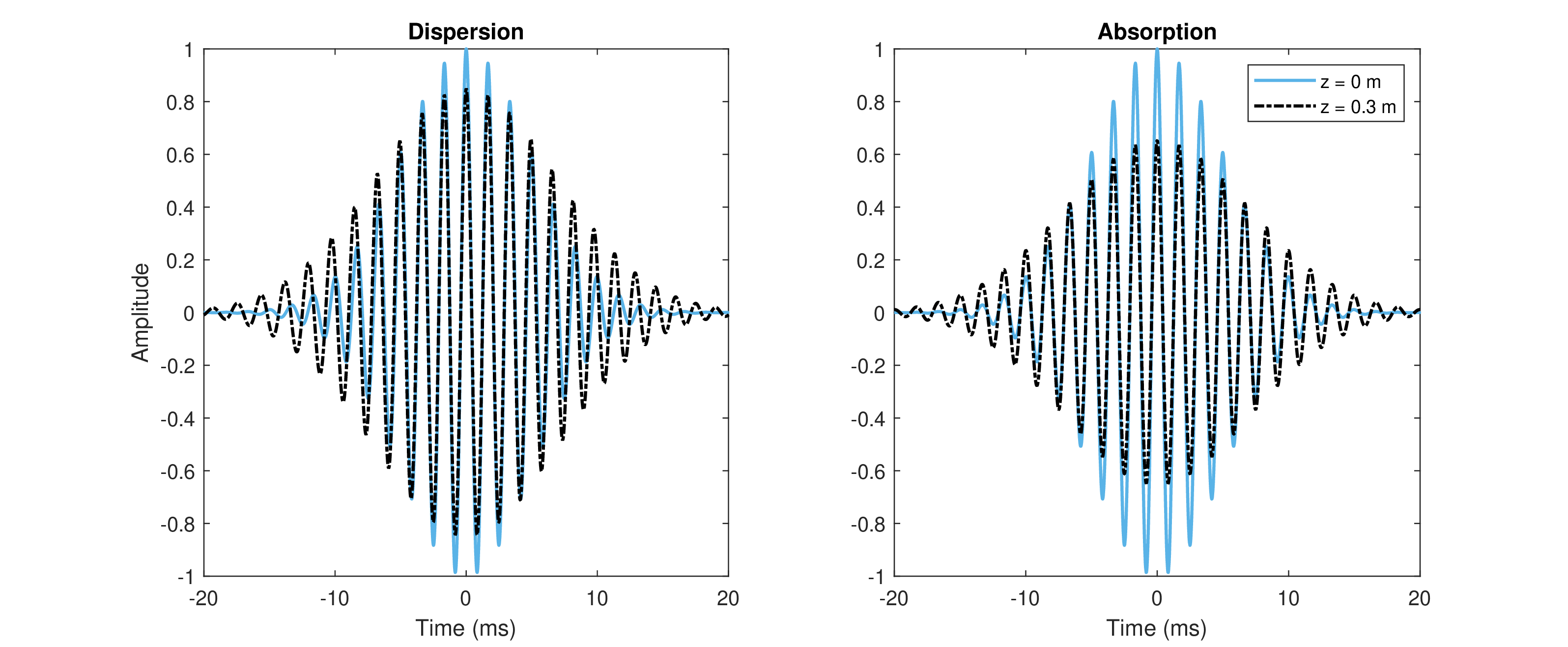
Figure B.1: An example of a Gaussian pulse at \(z=0\) (solid blue) following dispersion (left) and absorption (right) after moving 30 cm in space (dashed black), according to Eqs. (§B.10) and (§B.11) (real part). The figures show all features of group dispersion discussed in the text: reduced amplitude, broader pulse, and chirped phase. The chirp can be clearly seen by comparing the (phase) peak locations before and after the pulse (envelope) peak. While the phase appears in sync at \(t=0\), the periods are shorter at \(t<0\) and longer at \(t>0\). The parameters used for dispersion simulation are \(f_c = 600\) Hz, \(v_p = c = 343\) m/s, \(t_0=5\) ms, \(v_g=0.8c=274\) m/s, \(\beta”=0.00008\) s\(^2\)/m rad. For the absorption simulation the same pulse was used with \(\alpha_0 = -0.3i\) 1/m, and \(\alpha” = -0.00008i\) s\(^2\)/m rad.

B.2 Group-velocity absorption

Similar effects to dispersion are observed by an analogous manipulation of the absorption (Siegman, 1986; p. 335), which can be explored by examining a strictly imaginary dispersion relation \(k(\omega) = i\left[\alpha_0 + \alpha'(\omega- \omega_c) + \frac{\alpha”}{2}(\omega- \omega_c)^2 \right]\). Due to the similarity, absorption is sometimes referred to as gain dispersion, but with opposite signs (Siegman, 1986; 356-360; Haus, 1984; 283-287), so when any of the \(\alpha\)'s are positive, there is gain. In most cases (e.g., air, saturated media in lasers) \(\alpha'=0\) and only the quadratic effect is of interest. The solution to the paratonal equation §10.19 with Eq. §B.4 as input envelope is then a variation on Eq. §B.8

\[ p(z,t) = \frac{at_0}{\sqrt{t_0^2-\alpha” z}}\exp\left[i(\omega_c t-k_c z)+\alpha_0 z\right] \exp\left( -\frac{1}{2} \frac{t ^2 }{t_0^2-\alpha” z} \right) \,\,\,\,\,\,\, \alpha” < 0 \]

(B.11)

where the condition for negative \(\alpha”\) is necessary to make the Fourier transform solution method of §B.7 tractable. The effect on the amplitude of the pulse and the width are apparent directly from the equation without any additional transformation. A uniform attenuation is applied to the entire pulse, which is proportional to the distance, when \(\alpha_0<0\). A time/frequency-dependent loss broadens the pulse when \(\alpha”<0\), which also scales the amplitude of the pulse accordingly. An example of absorption is given on the right of Figure §B.1 for similar parameters to the above example. If \(\alpha' \neq 0\) then the phase would be affected as well, and manifest as a subtler chirp than the linear chirp caused by the quadratic dispersive terms. However, this can be compounded into a complex group velocity instead, so its effect is less critical. Unlike dispersion, absorption is accompanied by energy loss.

B.3 Complex pulse calculus

This section presents several useful formulas for working with complex Gaussian functions, which are used throughout the text. Additionally, it aims to provide some intuition for these functions—whether they are used as signal envelopes or as filters.

The fundamental sound pulse used in this work—the sound atom, or the logon—is the complex Gaussian function that modulates an arbitrary carrier. Its real part in the exponential represents the energy and width or the pulse, whereas the imaginary part imparts the signal with quadratic phase¹⁸⁶. Strictly speaking, the Gaussian makes for non-analytic signals, because it has a non-zero negative spectrum. Exactly the same functions are also used as filters in the imaging transforms that are employed throughout the text, which are similarly non-causal because they do not vanish at \(t<0\). Nevertheless, the complex Gaussian function enables closed-form solutions for all the relevant equations and is characterized by the same defining features as other relevant signals in analysis (Siegman, 1986; Blinchikoff and Zverev, 2001). Critically, it is the simplest second-order curved signal/filter that has a characteristic duration and chirp (curvature), which enables instantaneous amplitude and frequency modulations, respectively.

The general class of pulses we consider contains a chirp at the source, which is the simplest type of frequency modulation (FM). It is easy to see how it directly interacts with the group-velocity dispersion of the medium. Consider a signal with the complex envelope

\[ a(0,t) = a\exp \left( -\frac{t^2}{2t_0^2} + \frac{im_0t^2}{2} \right) \]

(B.12)

where \(m_0\) is the frequency velocity—the slope of the instantaneous frequency (Eq. §6.31) of the signal with envelope \(a(0,t)\). As before, we can obtain a full solution to the dispersion problem. For this purpose, it is convenient to make the following substitution¹⁸⁷ of a complex Gaussian width \(t'\),

\[ \frac{1}{t^{'2}} = \frac{1}{t_0^2} - im_0 = \frac{1-im_0 t_0^2}{t_0^2} \,\,\,\, \Rightarrow \,\,\,\, t^{'2} = \frac{t_0^2}{1-im_0 t_0^2} = t_0^2\frac{1+im_0 t_0^2}{1+m_0^2 t_0^4} \]

(B.13)

By using \(t'\) directly in Eq. §B.8, we can obtain the full signal at \(z\) after propagating through the dispersive medium

\[ p(z,t) = \frac{t_0^2(1 + im_0t_0^2)}{1+m^2t_0^4} \sqrt{\frac{t_0^2(1 + um_0) - i(2um_0^2t_0^4+m_0 t_0^4+2u)}{(1+2m_0u)^2t_0^4+4u^2}}\exp\left[i(\omega_c t-k_c z)\right] \\ \cdot \exp\left[-\frac{t_0^2(1 + um_0)}{(1+2m_0u)^2t_0^4+4u^2}\frac{\tau^2 }{2}\right] \exp\left[\frac{i(2um_0^2t_0^4+m_0 t_0^4+2u)}{(1+2m_0u)^2t_0^4+4u^2}\frac{\tau^2 }{2}\right] \]

(B.14)

which indicates that the dispersed chirp slope depends on \(m_0\), \(u\) and on \(t_0\) itself.

The eventual filtering as is given in Eqs. §B.14 and §B.11 is most readily treated as a multiplication of several Gaussian elements, which are then governed by relatively simple operations of scaling. This operation is also common in imperfect imaging, however, which is implicated by chirping as a result of defocus. Thus, we would like to find out how two arbitrary complex Gaussian functions of the form of Eq. §B.12 interact under multiplication. This is encountered in the (Fourier-transformed) convolution of the input envelope spectrum with the imaging system transfer function, or equivalently, when a temporal envelope is processed by a time-domain phase modulator (i.e., a time lens). Let us look at two complex Gaussians with constant amplitudes, \(a_1\) and \(a_2\), characterized by parameters \(t_1\) and \(m_1\), and \(t_2\) and \(m_2\), respectively, or the complex widths \(t'_1\) and \(t'_2\). The product of the two complex Gaussians is

\[ a_1(\tau)a_2(\tau) = a_1a_2\exp\left( -\frac{\tau^2}{2t_1^2} + \frac{im_1\tau^2}{2} \right)\exp\left( -\frac{\tau^2}{2t_2^2} + \frac{im_2\tau^2}{2} \right)\\ = a_1a_2\exp\left[ -\frac{(t_1^2 + t_2^2)}{2t_1^2 t_2^2}\tau^2 + \frac{i(m_1+m_2)}{2}\tau^2 \right] = a_1a_2\exp\left[ -\frac{(t_1^{'2} + t_2^{'2})}{2t_1^{'2} t_2^{'2}}\tau^2 \right] \]

(B.15)

Importantly, the third equality shows that the slopes of the linear chirps are additive under modulation, whereas for the pulse width, it is the reciprocal of the width squared that is additive.

Another recurrent operation on the envelope is scaling, where the pulse is being magnified by a factor \(M\) as a result of imaging. In this case, the envelope time variable is substituted by \(\tau/M\) (see Eq. §12.19)

\[ a\left(\frac{\tau}{M}\right) = \frac{a_0}{\sqrt{M}}\exp \left(-\frac{\tau^2}{2M^2t_0^{'2}} \right) = \frac{a_0}{\sqrt{M}}\exp\left( -\frac{\tau^2}{2M^2t_0^2} + \frac{im_0\tau^2}{2M^2} \right) \]

(B.16)

which means that the pulse is magnified, while its chirp rate is demagnified (for \(M>1\))

\[ t_0 \xrightarrow{\text{M}} Mt_0 \]

(B.17)

\[ m_0 \xrightarrow{\text{M}} \frac{m_0}{M^2} \]

(B.18)

\[ a_0 \xrightarrow{\text{M}} \frac{a_0}{\sqrt M} \]

(B.19)

where the last relation follows from the first one.

In some cases, the complex width \(t_1'\) of a particular transform is available numerically, but it is necessary to obtain the underlying width and chirp factors. Bringing it to the form of §B.13, this can be done using these expressions

\[ t_1 = \left[\Re\left(\frac{1}{t^{'2}_1}\right)\right]^{-\frac{1}{2}} \]

(B.20)

\[ m_1 = -\Im\left({\frac{1}{t_1^{'2}}}\right) \]

(B.21)

A common and somewhat more realistic linear FM pulse that is often employed (Levanon and Mozeson, 2004; p. 57) has a rectangular envelope of width \(T\)

\[ a(\tau) = \frac{a_0}{\sqrt{T}}\mathop{\mathrm{rect}} \left( \frac{t}{T} \right) \exp\left( i\pi m_r\tau^2 \right) \,\,\,\,\,\,\,\,\, m_r = \pm\frac{B}{T} \]

(B.22)

where the frequency slope \(m_r\) is by definition the quotient of the bandwidth \(B\) and pulse width \(T\). By comparing the coefficients of our complex pulse from Eq. §B.12, a simple transformation between the slopes can be obtained

\[ m_0 = 2\pi m_r = 2\pi\frac{B}{T} \]

(B.23)

This relation can provide some insight about the magnitude of \(m_0\) of the Gaussian pulse. When the pulse is made narrow, \(T \rightarrow 0\), its associated frequency velocity can be very large, depending on the bandwidth \(B\). If in addition the spectral bandwidth is made very large, \(B \rightarrow \infty\), the pulse functionally approximates a delta function in the temporal domain. Therefore, the closer the pulse is to a perfect impulse, the larger is its frequency velocity. If the impulse does not disperse much in propagation, then its impulse shape is retained, which means that it is experienced almost instantaneously across the spectrum.

Finally, depending on the application, the effective Gaussian pulse width has to be scaled to constrain its infinite support, but still preserve some of its characteristics. In photonics, pulses are customarily quantified using the full-width half maximum (FWHM) of the particular pulse function. It is defined with respect to the pulse power, using \(t_0\) as a parameter, so at half the peak amplitude (quarter the peak power) \(t = \mathop{\mathrm{FWHM}} \cdot t_{0}=2\sqrt{2\ln2}t_0\) (e.g., New, 2011, p. 120). See Figure §B.2 for illustration.

Another example is plotted in Figure §B.3 of complex Gaussian and rectangular pulses that have the same instantaneous frequency in the overlapping duration of the rectangular pulse. The Gaussian width is set to intersect the rect function so that the two pulses have equal power. Note that it is impossible to have the total pulse power, the peak amplitude, and the half power simultaneously equalized.

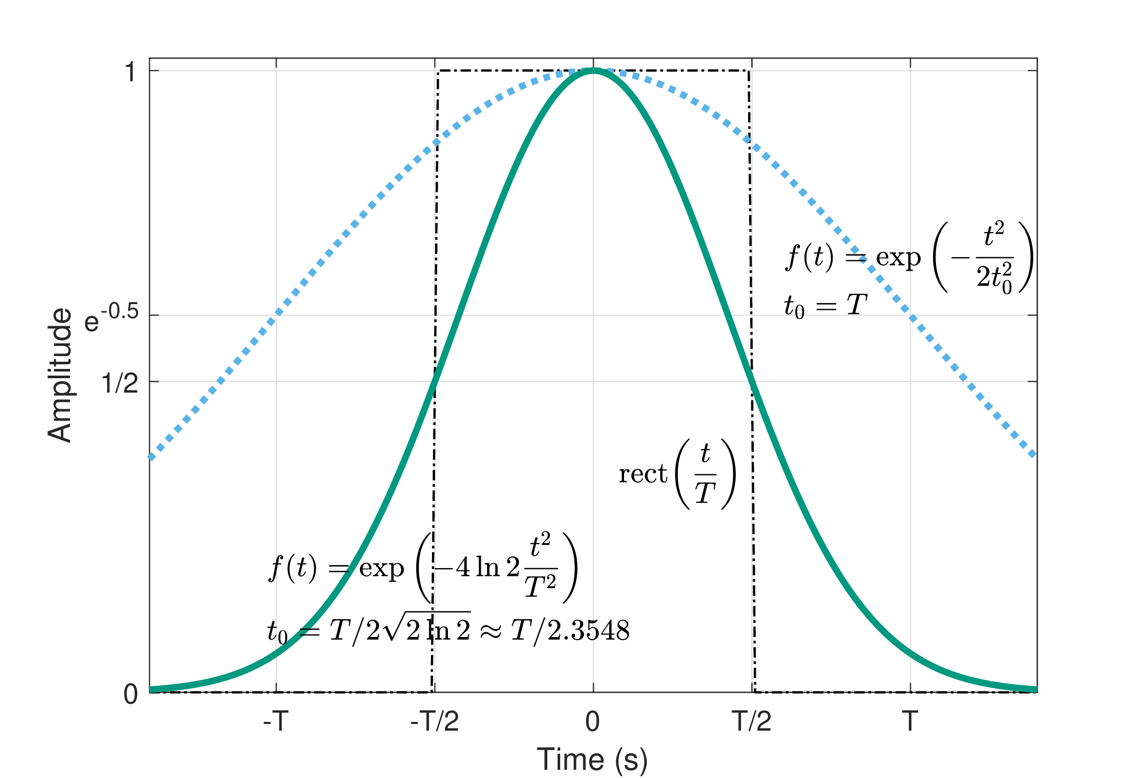
Figure B.2: A rectangular pulse (dash-dot black) of duration T and two Gaussian pulses of different widths \(t_0\) relative to T. The amplitude and time are given in arbitrary units, so that the rectangular pulse has an area of T, whereas the Gaussian pulses are not normalized. The broad Gaussian in dotted blue has the standard width of \(2t_0^2\) in the denominator of the exponent, which indicates that when \(t=T\), the amplitude drops to \(1/\sqrt{e}\) and the intensity to \(1/e\). Typically, this is not useful when working with \(t_0\), so it is preferable to convert it to equivalent rectangular duration, which is measured across both the negative and positive support of the pulse. The standard rectangular pulse and the Gaussian that intersects with it at \(T/2\) have the same width. Then, the conversion between the two is given by the FWHM.

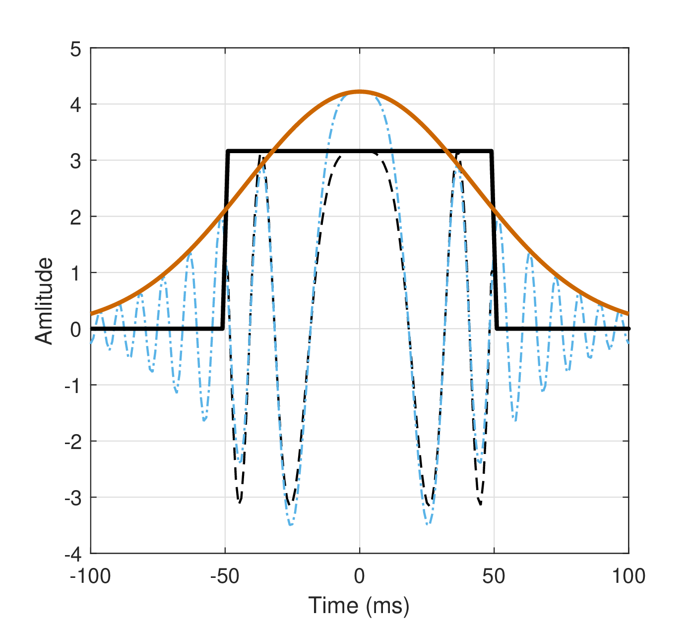
Figure B.3: Rectangular and Gaussian pulses that have the same instantaneous frequency in the overlapping duration, according to the substitutions in Eqs. §B.22 and §B.23, where \(B = 150\) Hz and \(T = 0.1\) s (of the full rectangular width). The Gaussian has a \(t_0 = T/(2 \sqrt{2\ln 2})\). In this example, the pulses are normalized to have equal total equal power.

Footnotes

182. Note that the term signal velocity is used in the context of waveguide analysis in Morse and Ingard (1968, p. 479), but with a non-standard interpretation. For Morse & Ingard the signal velocity is the velocity of the front of the wave, which has to be \(c\). However, these are two separate quantities in Brillouin (1960) and elsewhere, where the signal velocity is not equal to the front velocity, but to the group velocity, unless the medium is dispersionless.

183. Note that sometimes the inverse is done, by expanding \(\omega(k)\) around \(k_c\) (Eq. §3.8 and Elmore and Heald, 1969; pp. 431–435). We shall stick with the formalism found in optics, as is also advocated in Lighthill (1965).

184. This term has not been imported to acoustics, to the best knowledge of the author, except for acoustic measurements of tubes in Latif et al. (2000). Another near-mention may have been in the context of acoustic dispersion in waveguides. In their analysis of the phase and group velocities of acoustic waveguides, Morse and Ingard (1968, pp. 477–478) expounded on a similar problem as presented here of a Gaussian pulse propagating in one-dimension, over the fundamental (plane wave) mode of the tube. However, even though an absorptive “frequency spread” term appeared in their Taylor expansion of \(k\) (as in Eq. §B.1), they unfortunately neglected it in their subsequent analysis and discussion, so GVD never came about. GVD is commonly used in optics and fiber optics (e.g., Agrawal, 2001; New, 2011).

185. From Merriam-Webster's dictionary: https://www.merriam-webster.com/dictionary/para.

186. Note that unlike Gabor's logons (Gabor, 1946), the envelope used here is complex rather than real.

187. A similar approach was developed by Siegman (1986, Chapter 9), where a complex Gaussian parameter was defined as \(\Gamma \equiv a-ib\), where \(a=1/2t_0^2\) denotes the width and \(b\) denotes frequency slope. A geometrical representation of \(\Gamma\) is then investigated in the spectral domain, as a function of dispersion and the resultant pulse compression.

References

Agrawal, Govind P. Nonlinear Fiber Optics. Academic Press, 3rd edition, 2001.

Brillouin, Léon. Wave Propagation and Group Velocity. Academic Press, Inc., 1960.

Elmore, William C. and Heald, Mark A. Heald, MA. McGraw-Hill, Inc., 1969.

Gabor, Dennis. Theory of communication. Part 1: The analysis of information. Journal of the Institution of Electrical Engineers-Part III: Radio and Communication Engineering, 93 (26): 429–457, 1946.

Haus, Hermann A. Waves and Fields in Optoelectronics. Prentice-Hall Inc., Englewood Cliffs, NJ, 1984.

Latif, R, Aassif, E, Maze, G, Decultot, D, Moudden, A, and Faiz, B. Analysis of the circumferential acoustic waves backscattered by a tube using the time-frequency representation of Wigner-Ville. Measurement Science and Technology, 11 (1): 83, 2000.

Levanon, Nadav and Mozeson, Eli. Radar Signals. John Wiley & Sons, Inc., Hoboken, NJ, 2004.

Lighthill, MJ. Group velocity. Journal of the Institute of Mathematics and its Applications, 1: 1–28, 1965.

Morse, Philip M. and Ingard, K. Uno. Theoretical Acoustics. Princeton University Press, Princeton, NJ, 1968.

New, Geoffrey. Introduction to Nonlinear Optics. Cambridge University Press, 2011.

Siegman, Anthony E. Lasers. University Science Books, Mill Valley, CA, 1986.

Toll, John S. Causality and the dispersion relation: Logical foundations. Physical Review, 104 (6): 1760, 1956.

Blinchikoff, Herman J. and Zverev, Anatol I. Filtering in the time and frequency domains. Scitech Publishing Inc., Rayleigh, NC, 2001.